


Idiomas
Páginas
Jurídico


ESCUELA POLITÉCNICA SUPERIOR DE MONDRAGON
UNIBERTSITATEA MONDRAGON UNIBERTSITATEKO GOI ESKOLA POLITEKNIKOA
MONDRAGON UNIVERSITY FACULTY OF ENGINEERING
Trabajo fin de grado presentado para la obtención del título de Titulua eskuratzeko gradu bukaerako lana
Final degree project for taking the degree of
MÁSTER UNIVERSITARIO EN INGENIERÍA INDUSTRIAL. INDUSTRIA INGENIARITZAKO UNIBERTSITATE MASTERRA
MASTER IN INDUSTRIAL ENGINEERING
Título del Trabajo Lanaren izenburua Project Topic
HYSTERETIC AND DAMAGE EFFECTS MODELLING FOR
COMPOSITE MATERIALS BY FRACTIONAL MODELS:
STRAIN RATE EFFECTS
Autor Egilea Author DIEGO ERRANDONEA GONZALEZ Curso Ikasturtea Year 2014/2015

Título del Trabajo Lanaren izenburua Project Topic
HYSTERETIC AND DAMAGE EFFECTS MODELLING FOR
COMPOSITE MATERIALS BY FRACTIONAL MODELS:
STRAIN RATE EFFECTS
Nombre y apellidos del autor Egilearen izen-abizenak
Author's name and surnames
ERRANDONEA GONZALEZ, DIEGO
Nombre y apellidos del/los director/es del trabajo Zuzendariaren/zuzendarien izen-abizenak
Project director's name and surnames
GORNET, LAURENT
MATEOS, MODESTO
Lugar donde se realiza el trabajo Lana egin deneko lekua
Company where the project is being developed
ECOLE CENTRALE DE NANTES
Curso académico Ikasturtea
Academic year
2014/2015
El autor/la autora del Trabajo Fin de Grado, autoriza a la Escuela Politécnica Superior de Mondragon
Unibertsitatea, con carácter gratuito y con fines exclusivamente de investigación y docencia, los derechos de reproducción
y comunicación pública de este documento siempre que: se cite el autor original, el uso que se haga de la obra no sea comercial y no se
cree una obra derivada a partir del original. Gradu Bukaerako Lanaren egileak, baimena ematen dio Mondragon Unibertsitateko Goi Eskola Politeknikoari Gradu Bukaerako Lanari
jendeaurrean zabalkundea emateko eta erreproduzitzeko; soilik ikerketan eta hezkuntzan erabiltzeko eta doakoa izateko baldintzarekin.
Baimendutako erabilera honetan, egilea nor den azaldu beharko da beti, eragotzita egongo da erabilera komertziala baita lan
originaletatik lan berriak eratortzea ere

iii
ABSTRACT
This project deals with the modeling of composite materials by fractional models
taking into account hysteretic and damage effects as well as strain rate effects.
The main objective of this project has been the development of a viscous matlab
model for composite materials which calculates the behavior of the material with less
computational effort.
For this, a previous deep study and achievement of knowledge about Fractional
derivatives, viscous rheological models has been done.
Afterwards, a design of a Matlab program subroutine has been made, which
implements Fractional Derivatives. First, an example with a simple function which
calculates the fractional derivative has been developed. This program has been compared
with the results obtained by hand in order to validate the model and with the purpose of
implement it in next real cases.
Secondly, this method has been implemented in real cases to calculate the stress
in a specific material. Two different situations has been solved, one with a linear
deformation and other with a constant deformation.
Finally, a deeper study of the error, which this numerical method involves has
been done in order to find a balance between the precision of the calculus and the
computational effort.
The results show that the method proposed will be interesting to use in the future.
iv
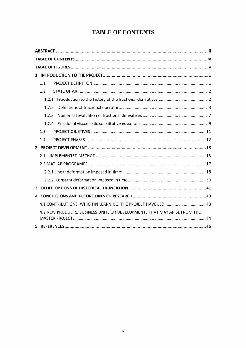
TABLE OF CONTENTS
ABSTRACT .......................................................................................................................... iii
TABLE OF CONTENTS........................................................................................................... iv
TABLE OF FIGURES ............................................................................................................... v
1 INTRODUCTION TO THE PROJECT ..................................................................................... 1
1.1 PROJECT DEFINITION ..................................................................................................... 1
1.2 STATE OF ART ................................................................................................................ 2
1.2.1 Introduction to the history of the fractional derivatives ........................................... 2
1.2.2 Definitions of fractional operator .............................................................................. 3
1.2.3 Numerical evaluation of fractional derivatives ......................................................... 7
1.2.4 Fractional viscoelastic constitutive equations ........................................................... 9
1.3 PROJECT OBJETIVES ..................................................................................................... 11
1.4 PROJECT PHASES ......................................................................................................... 12
2 PROJECT DEVELOPMENT ............................................................................................... 13
2.1 IMPLEMENTED METHOD ................................................................................................ 13
2.2 MATLAB PROGRAMES ....................................................................................................... 17
2.2.1 Linear deformation imposed in time: ........................................................................ 18
2.2.2. Constant deformation imposed in time .................................................................... 30
3 OTHER OPTIONS OF HISTORICAL TRUNCATION .............................................................. 41
4 CONCLUSIONS AND FUTURE LINES OF RESEARCH ........................................................... 43
4.1 CONTRIBUTIONS, WHICH IN LEARNING, THE PROJECT HAVE LED .................................... 43
4.2 NEW PRODUCTS, BUSINESS UNITS OR DEVELOPMENTS THAT MAY ARISE FROM THE
MASTER PROJECT .................................................................................................................... 44
5 REFERENCES .................................................................................................................. 46

v
TABLE OF FIGURES
Figure 1: Comparison of two numerical methods made by hand............................................... 15
Figure 2: Comparison of two numerical methods with Matlab program. .................................. 15
Figure 3: Particular case for fractional derivative. ..................................................................... 17
Figure 4: Linear deformation input. ........................................................................................... 18
Figure 5: Alpha=1 for linear input. ............................................................................................ 20
Figure 6: Error for alpha=1. ....................................................................................................... 21
Figure 7: Alpha=0.999 for linear input. ..................................................................................... 21
Figure 8: Alpha=0.95 for linear input. ....................................................................................... 22
Figure 9: Alpha=0.9 for linear input. ......................................................................................... 22
Figure 10: 100 points of the historical ....................................................................................... 23
Figure 11: Error of 100 points .................................................................................................... 23
Figure 12: 50 points of the historical ......................................................................................... 24
Figure 13: error of 50 points ...................................................................................................... 24
Figure 14: Errors for alpha=0.99 linear input ............................................................................ 25
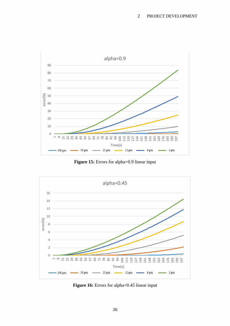
Figure 15: Errors for alpha=0.9 linear input .............................................................................. 26
Figure 16: Errors for alpha=0.45 linear input ............................................................................ 26
Figure 17: Error for alpha=0.2845 linear input .......................................................................... 27
Figure 18: Error for alpha=0.225 linear input ............................................................................ 27
Figure 19: Error for alpha=0.10 linear input .............................................................................. 28
Figure 20: Error for alpha=0.05 linear input .............................................................................. 28
Figure 21: Evolution of the error for different alpha ................................................................. 29
Figure 22: range of the curves for all the alpha .......................................................................... 30
Figure 23: input of deformation applied .................................................................................... 31
Figure 24: Alpha=0.999 for constant input deformation ............................................................ 33
Figure 25: Alpha=0.9 for constant input deformation ................................................................ 33
Figure 26: Error for all historical taken into account ................................................................. 34
Figure 27: 50 points for constant input ...................................................................................... 34
Figure 28: Error for 50 points constant input ............................................................................. 35
Figure 29: Error for alpha=0.999 constant input ........................................................................ 35
Figure 30: Error for alpha=0.99 constant input .......................................................................... 36
Figure 31: Error for alpha=0.9 constant input ............................................................................ 36
Figure 32: Error for alpha=0.45 constant input .......................................................................... 37
Figure 33: Error for alpha=0.2845 constant input ...................................................................... 37
Figure 34: Error for alpha=0.225 constant input ........................................................................ 38
Figure 35: Error for alpha=0.10 for constant input .................................................................... 38
Figure 36: Error for alpha=0.05 for constant input .................................................................... 39
Figure 37: Range of the curves for all the alpha ........................................................................ 39
Figure 38: Evolution of the error for different alpha ................................................................. 40
Figure 39: First method to calculate the fractional derivative.................................................... 41
Figure 40: Second method to calculate the fractional derivative ............................................... 41
Figure 41: Third method to calculate the fractional derivative .................................................. 42
2. INTRODUCTION TO THE PROJECT
1
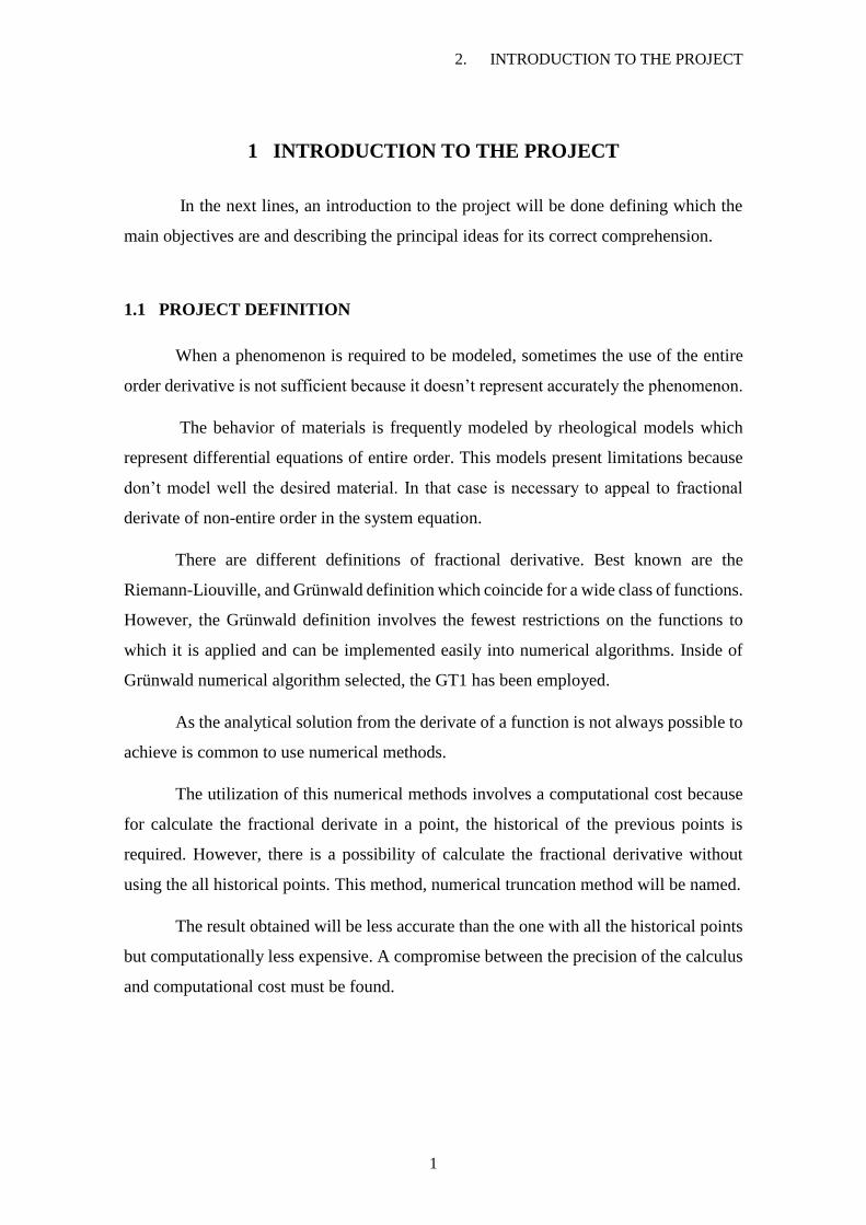
1 INTRODUCTION TO THE PROJECT
In the next lines, an introduction to the project will be done defining which the
main objectives are and describing the principal ideas for its correct comprehension.
1.1 PROJECT DEFINITION
When a phenomenon is required to be modeled, sometimes the use of the entire
order derivative is not sufficient because it doesn’t represent accurately the phenomenon.
The behavior of materials is frequently modeled by rheological models which
represent differential equations of entire order. This models present limitations because
don’t model well the desired material. In that case is necessary to appeal to fractional
derivate of non-entire order in the system equation.
There are different definitions of fractional derivative. Best known are the
Riemann-Liouville, and Grünwald definition which coincide for a wide class of functions.
However, the Grünwald definition involves the fewest restrictions on the functions to
which it is applied and can be implemented easily into numerical algorithms. Inside of
Grünwald numerical algorithm selected, the GT1 has been employed.
As the analytical solution from the derivate of a function is not always possible to
achieve is common to use numerical methods.
The utilization of this numerical methods involves a computational cost because
for calculate the fractional derivate in a point, the historical of the previous points is
required. However, there is a possibility of calculate the fractional derivative without
using the all historical points. This method, numerical truncation method will be named.
The result obtained will be less accurate than the one with all the historical points
but computationally less expensive. A compromise between the precision of the calculus
and computational cost must be found.

1. INTRODUCTION TO THE PROJECT
2
1.2 STATE OF ART
Numerical methods are a simple and useful tool for obtaining a good curve fitting
when working with any type of behavior models. ‘Least squares fit’, for example is one
of the most used nowadays for these type of approximations, nevertheless this method
does not always provide a good fitting, that is why other numerical or mathematical
methods had been developed.
Since 1921, some mathematicians and investigators have observed that stress
relaxation of some materials might be modeled by fractional powers of time and stated
that the stiffness and damping properties of viscoelastic materials are fit much better by
using fractional powers. Those investigations where the beginning of the materials
behavior Modelling using fractional derivatives.
1.2.1 Introduction to the history of the fractional derivatives
The history of fractional derivatives can be dated back to 1695, when L´Hôpital
and Leibniz were communicating whether it made sense to define an operator d𝑛/d𝑡𝑛 for
𝑛 = 1/2 [1]. In the 18th century there were only few contributions to this topic and it was
Euler who again raised the question of a derivative of order 𝑛 for 𝑛 being a fraction. In
1819 Lacroix first mentioned derivatives of arbitrary order in a text [2]. The first
application of fractional derivatives was given in 1823 by Abel [3] who applied the
fractional calculus in the solution of an integral equation that arises in the formulation of
the tautochrone problem. Later, Liouville attempted to give a logical definition of
fractional derivatives [4-6]. One can state that the whole theory of fractional derivatives
and integrals was established in the 2nd half of the 19th century. Further names to be
mentioned are Grünwald, Krug, Riemann, and Letnikov. A more detailed overview
concerning the history of fractional derivatives in general is given in [7]. However, the
term fractional integrodifferential operator is misleading as it implies that only rational
numbers as orders of derivatives or integrals are defined. In fact, the order of derivatives
or integrals may be any real number; even for complex numbers fractional derivatives are
defined.

1. INTRODUCTION TO THE PROJECT
3
In 1921 Nutting [8] observed that stress relaxation of some materials might be
modeled by fractional powers of time and Gemant stated that the stiffness and damping
properties of viscoelastic materials are fit much better by using fractional powers of
frequency. The latter was the first who suggested explicitly to use fractional derivatives
in the constitutive equation [9, 10].
In 1949 Scott-Blair [11] again suggested the application of fractional time-
derivatives to meet the observations of Nutting and Gemant. Caputo and Mainardi [12,
13] also found good agreement with experimental results when using fractional
derivatives for the description of viscoelastic materials. Up to the beginning of the 1980s,
the concept of fractional derivatives in conjunction with viscoelasticity had to be seen as
a sort of curve-fitting method. Then, Bagley and Torvik [14] gave a physical justification
for this concept. Starting point is the molecular theory of Rouse, later modified by Ferry,
resulting in fractional derivatives of order ½ in the shear stress-strain relation. Similar
considerations for the molecular theory of Zimm lead to fractional derivative of order 2/3.
Bagley and Torvik also developed constraints for the fractional 3-parameter
model, ensuring the model to predict a non-negative rate of energy dissipation and
internal work [15]. The implementation of fractional constitutive equations of differential
operator type into FE formulations was studied substantially by Padovan [16]. Hereditary
integral fractional constitutive equations were investigated by Koeller [17] and their
implementation into FE formulations is demonstrated by Enelund and Josefson [18].
Enelund et al. studied the FE implementation of fractional derivative viscoelastic
formulations using the concept of internal variables [19]. Implementations of fractional
constitutive equations into the BEM were investigated by Gaul and Schanz [20] for the
time domain and by Gaul [21 - 23] for the frequency domain, respectively.
1.2.2 Definitions of fractional operator
There are different definitions of fractional derivatives. Best known are the
Riemann-Liouville and the Grünwald definition which coincide for a wide class of
functions, see e.g. [24]. However, the Grünwald definition involves the fewest restrictions
on the functions to which it is applied and can be implemented easily into numerical
algorithms. For that reason Grünwald definition which has been applied is going to be
explained in the following part.

1. INTRODUCTION TO THE PROJECT
4
Grünwald Definition of Fractional Derivatives
Starting point is the definition of the first (integer-order) time derivative in terms of a
backward difference quotient
d1𝑓(𝑡)
d1= lim
𝛥𝑡→0
𝑓(𝑡) − 𝑓(𝑡 − 𝛥𝑡)
𝛥𝑡 ( 1)
Repeated application leads to
d2𝑓(𝑡)
d2= lim
𝛥𝑡→0
𝑓(𝑡) − 2𝑓(𝑡 − 𝛥𝑡) + 𝑓(𝑡 − 2𝛥𝑡)
(𝛥𝑡)2 ( 2)
d3𝑓(𝑡)
d3= lim
𝛥𝑡→0
𝑓(𝑡) − 3𝑓(𝑡 − 𝛥𝑡) + 3 𝑓(𝑡 − 2𝛥𝑡) − 𝑓(𝑡 − 3𝛥𝑡)
(𝛥𝑡)3 ( 3)
That can be written for any integer-order derivative as
d𝑛𝑓(𝑡)
d𝑡𝑛= lim
𝛥𝑡→0[(𝛥𝑡)−𝑛 ∑(−1)𝑗 (
𝑛
𝑗) 𝑓(𝑡 − 𝑗𝛥𝑡)
𝑛
𝑗=0
] ( 4)
Where the binomial coefficient
(𝑛
𝑗) = {
𝑛!
𝑗! (𝑛 − 𝑗)! 𝑓𝑜𝑟 0 ≤ 𝑗 ≤ 𝑛,
0, 𝑓𝑜𝑟 0 ≤ 𝑛 < 𝑗,
( 5)
Is used. If we replace the time step 𝛥𝑡 by the fraction t/N, N = 1, 2, 3…., Equation (4)
can be written as
d𝑛𝑓(𝑡)
d𝑡𝑛= lim
𝑁→∞[(
𝑡
𝑁)−𝑛
∑(−1)𝑗 (𝑛
𝑗) 𝑓 (𝑡 − 𝑗
𝑡
𝑁)
𝑁−1
𝑗=0
] ( 6)
Noting that
(𝑛
𝑗) = 0 for 𝑗 > 𝑛 ( 7)

1. INTRODUCTION TO THE PROJECT
5
The upper limit of the sum N-1 seems to be somewhat arbitrary. However, it
derives from defining the lower limit of an integral, when (6) is used to define integrals
as a limit of a Riemann sum, see [22 - 24].
In order to deduce a formulation that is valid for any real order derivative we use
the extended definition of the binomial coefficient
(𝑎
𝑗) = {
𝑎(𝑎 − 1)(𝑎 − 2)… (𝑎 − 𝑗 + 1)
𝑗! 𝑓𝑜𝑟 𝑗 > 0,
1, 𝑓𝑜𝑟 𝑗 = 0,
( 8)
Wherein a is real and j is a natural number. For 𝑗 > 0 the expression (−1)𝑗 (𝑛𝑗)
can be written as
(−1)𝑗 (𝑛
𝑗) = (−1)𝑗
𝑛(𝑛 − 1)(𝑛 − 2)… (𝑛 − 𝑗 + 2)(𝑛 − 𝑗 + 1)
𝑗! } 𝑗 𝑓𝑎𝑐𝑡𝑜𝑟𝑠
= (𝑗 − 𝑛 − 1)(𝑗 − 𝑛 − 2)… (−𝑛 + 1)(−𝑛)
𝑗!
Such that 𝛤 is the gamma function. For j = 0 Equation (9) of course holds as well.
Inserting (9) into (6), we obtain
d𝑛𝑓(𝑡)
d𝑡𝑛= lim
𝑁→∞[(
𝑡
𝑁)−𝑛
∑𝛤(𝑗 − 𝑛)
𝛤(−𝑛)𝛤(𝑗 + 1)𝑓 (𝑡 − 𝑗
𝑡
𝑁)
𝑁−1
𝑗=0
] ( 10)
Which is valid for any real-order derivative (n > 0). If we now reinterpret n to be
any real number α, the Gr�̈�nwald definition [14] of fractional derivatives (and integrals)
is derived
d𝛼𝑓(𝑡)
d𝑡𝛼= lim
𝑁→∞[(
𝑡
𝑁)−𝛼
∑ 𝐴𝑗+1𝑓 (𝑡 − 𝑗𝑡
𝑁)
𝑁−1
𝑗=0
] ( 11)
Wherein
𝐴𝑗+1 ≡𝛤(𝑗 − 𝑛)
𝛤(−𝑛)𝛤(𝑗 + 1) ( 12)
Are the so called Grünwald coefficients 𝐴𝑗+1 .
(−1)𝑗 (𝑛
𝑗) = (
𝑗 − 𝑛 − 1
𝑗) ≡
𝛤(𝑗 − 𝑛)
𝛤(−𝑛)𝛤(𝑗 + 1) ( 9)

1. INTRODUCTION TO THE PROJECT
6
As indicated above, Equation (10) is also valid for integer-order integrals, as can
be seen directly from the Riemann definition of an integral, where the lower limit is taken
to be zero.
In this case n ranges from 0 to −∞ and Equation (11) can be interpreted as a
definition of either fractional integrals and derivatives, where α ranges from −∞ to ∞.
Note in this context, that all Grünwald coefficients 𝐴𝑗+1 are different from zero as
long as the order of derivative 𝛼 is not a positive integer. If e.g.,𝛼 = −1, then 𝐴𝑗+1 = 1
for all 𝑗, according to the Riemann sum.
For 𝛼 being a natural number 𝑛, only the first 𝑛 + 1 Grünwald coefficients 𝐴𝑗+1
are non zero, indicating a local operator. On the other hand, as for any positive non-integer
number all coefficients 𝐴𝑗+1 are non-zero, fractional derivatives are non-local operators,
except for integer-order derivatives. Analogous to the fractional integral, the lower limit
(also called ‘terminal’) of the fractional derivative in (11) is zero. This is indicated by the
function values taken into account in the sum in Equation (11), i.e. the first addend (j =
0) is 𝐴1 𝑓(𝑡) and the last 𝑗 = 𝑁 − 1 is
𝐴𝑁 𝑓 (𝑡 −𝑁 − 1
𝑁𝑡) = 𝐴𝑁 𝑓 (
𝑡
𝑁). ( 13)
Thus, the interval (0, 𝑡] is divided into 𝑁 sections of equal size for the calculation
of the fractional derivative or integral.
In this paper, the lower terminal is assumed to be zero. This may be indicated
using the differential operator representation
𝐷0 𝑡𝛼 =
d𝛼𝑓(𝑡)
d𝑡𝛼= lim
𝑁→∞[(
𝑡
𝑁)−𝛼
∑ 𝐴𝑗+1𝑓 (𝑡 − 𝑗𝑡
𝑁)
𝑁−1
𝑗=0
].
( 14)
Mathematically, the lower terminal defines the instant of the time from after which
the ‘history’ of a function 𝑓(𝑡) is taken into account, similar to ordinary integrals. In
Section 4, fractional derivatives are applied to stresses and strains in order to describe the
viscoelastic material behavior. Thus, if a vicoelastic structure is considered which is
completely relaxed before the beginning of loading after time 𝑡 = 0, the whole
deformation history is taken into account by Equation (14) and all initial conditions are
zero.
1. INTRODUCTION TO THE PROJECT
7
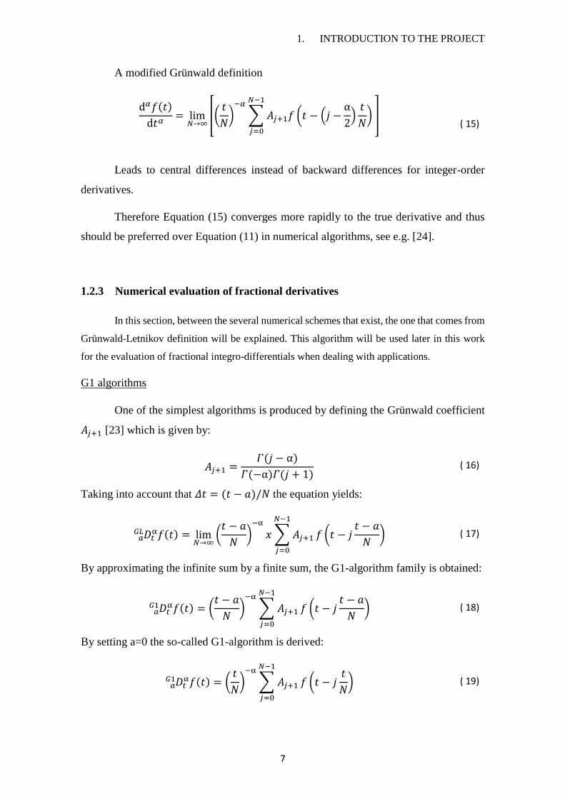
A modified Grünwald definition
d𝛼𝑓(𝑡)
d𝑡𝛼= lim
𝑁→∞[(
𝑡
𝑁)−𝛼
∑ 𝐴𝑗+1𝑓 (𝑡 − (𝑗 −α
2)
𝑡
𝑁)
𝑁−1
𝑗=0
]
( 15)
Leads to central differences instead of backward differences for integer-order
derivatives.
Therefore Equation (15) converges more rapidly to the true derivative and thus
should be preferred over Equation (11) in numerical algorithms, see e.g. [24].
1.2.3 Numerical evaluation of fractional derivatives
In this section, between the several numerical schemes that exist, the one that comes from
Grünwald-Letnikov definition will be explained. This algorithm will be used later in this work
for the evaluation of fractional integro-differentials when dealing with applications.
G1 algorithms
One of the simplest algorithms is produced by defining the Grünwald coefficient
𝐴𝑗+1 [23] which is given by:
𝐴𝑗+1 =𝛤(𝑗 − α)
𝛤(−α)𝛤(𝑗 + 1) ( 16)
Taking into account that 𝛥𝑡 = (𝑡 − 𝑎)/𝑁 the equation yields:
𝐷𝑎𝐺𝐿
𝑡α𝑓(𝑡) = lim
𝑁→∞(𝑡 − 𝑎
𝑁)−α
𝑥 ∑ 𝐴𝑗+1
𝑁−1
𝑗=0
𝑓 (𝑡 − 𝑗𝑡 − 𝑎
𝑁) ( 17)
By approximating the infinite sum by a finite sum, the G1-algorithm family is obtained:
𝐷𝑎𝐺1
𝑡α𝑓(𝑡) = (
𝑡 − 𝑎
𝑁)−α
∑ 𝐴𝑗+1
𝑁−1
𝑗=0
𝑓 (𝑡 − 𝑗𝑡 − 𝑎
𝑁) ( 18)
By setting a=0 the so-called G1-algorithm is derived:
𝐷𝑎𝐺1
𝑡α𝑓(𝑡) = (
𝑡
𝑁)−α
∑ 𝐴𝑗+1
𝑁−1
𝑗=0
𝑓 (𝑡 − 𝑗𝑡
𝑁) ( 19)
1. INTRODUCTION TO THE PROJECT
8
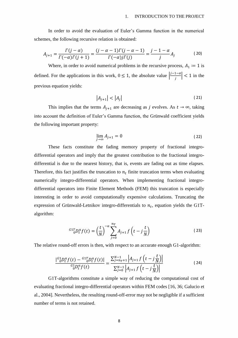
In order to avoid the evaluation of Euler’s Gamma function in the numerical
schemes, the following recursive relation is obtained:
𝐴𝑗+1 =𝛤(𝑗 − 𝛼)
𝛤(−𝛼)𝛤(𝑗 + 1)=
(𝑗 − 𝛼 − 1)𝛤(𝑗 − 𝛼 − 1)
𝛤(−𝛼)𝑗𝛤(𝑗)=
𝑗 − 1 − 𝛼
𝑗𝐴𝑗 ( 20)
Where, in order to avoid numerical problems in the recursive process, 𝐴1 ≔ 1 is
defined. For the applications in this work, 0 ≤ 1, the absolute value |𝑗−1−𝛼
𝑗| < 1 in the
previous equation yields:
|𝐴𝑗+1| < |𝐴𝑗| ( 21)
This implies that the terms 𝐴𝑗+1 are decreasing as 𝑗 evolves. As 𝑡 → ∞, taking
into account the definition of Euler’s Gamma function, the Grünwald coefficient yields
the following important property:
lim𝑗→∞
𝐴𝑗+1 = 0 ( 22)
These facts constitute the fading memory property of fractional integro-
differential operators and imply that the greatest contribution to the fractional integro-
differential is due to the nearest history, that is, events are fading out as time elapses.
Therefore, this fact justifies the truncation to 𝑛𝑡 finite truncation terms when evaluating
numerically integro-differential operators. When implementing fractional integro-
differential operators into Finite Element Methods (FEM) this truncation is especially
interesting in order to avoid computationally expensive calculations. Truncating the
expression of Grünwald-Letnikov integro-differentials to 𝑛𝑡, equation yields the G1T-
algorithm:
𝐷0𝐺1𝑇
𝑡α𝑓(𝑡) = (
𝑡
𝑁)−α
∑𝐴𝑗+1
𝑛𝑇
𝑗=0
𝑓 (𝑡 − 𝑗𝑡
𝑁) ( 23)
The relative round-off errors is then, with respect to an accurate enough G1-algorithm:
| 𝐷0𝐺1
𝑡α𝑓(𝑡) − 𝐷0
𝐺1𝑇𝑡α𝑓(𝑡)|
𝐷0𝐺1
𝑡α𝑓(𝑡)
=∑ |𝐴𝑗+1 𝑓 (𝑡 − 𝑗
𝑡𝑁)|𝑁−1
𝑗=𝑛𝑇+1
∑ |𝐴𝑗+1 𝑓 (𝑡 − 𝑗𝑡𝑁)|𝑁−1
𝑗=0
( 24)
G1T-algorithms constitute a simple way of reducing the computational cost of
evaluating fractional integro-differential operators within FEM codes [16, 36; Galucio et
al., 2004]. Nevertheless, the resulting round-off-error may not be negligible if a sufficient
number of terms is not retained.
1. INTRODUCTION TO THE PROJECT
9
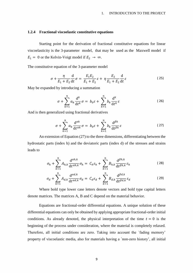
1.2.4 Fractional viscoelastic constitutive equations
Starting point for the derivation of fractional constitutive equations for linear
viscoelasticity is the 3-parameter model, that may be used as the Maxwell model if
𝐸1 = 0 or the Kelvin-Voigt model if 𝐸2 → ∞.
The constitutive equation of the 3-parameter model
𝜎 +𝜂
𝐸1 + 𝐸2
d
d𝑡𝜎 =
𝐸1𝐸2
𝐸1 + 𝐸2𝜀 + 𝜂
𝐸2
𝐸1 + 𝐸2
d
d𝑡𝜀 ( 25)
May be expanded by introducing a summation
𝜎 + ∑ 𝑎𝑘
𝑛
𝑘=1
d𝑘
d𝑡𝑘𝜎 = 𝑏0𝜀 + ∑ 𝑏𝑘
𝑛
𝑘=1
d𝑘
d𝑡𝑘𝜀 ( 26)
And is then generalized using fractional derivatives
𝜎 + ∑ 𝑎𝑘
𝑛
𝑘=1
d𝛼𝑘
d𝑡𝛼𝑘𝜎 = 𝑏0𝜀 + ∑ 𝑏𝑘
𝑛
𝑘=1
d𝛽𝑘
d𝑡𝛽𝑘𝜀 ( 27)
An extension of Equation (27) to the three dimensions, differentiating between the
hydrostatic parts (index h) and the deviatoric parts (index d) of the stresses and strains
leads to
𝜎ℎ + ∑ 𝐴ℎ,𝑘
𝑛
𝑘=1
d𝛼ℎ,𝑘
d𝑡𝛼ℎ,𝑘𝜎ℎ = 𝐶ℎ𝜀ℎ + ∑ 𝐵ℎ,𝑘
𝑛
𝑘=1
d𝛽ℎ,𝑘
d𝑡𝛽ℎ,𝑘𝜀ℎ ( 28)
𝜎𝑑 + ∑ 𝐴𝑑,𝑘
𝑛
𝑘=1
d𝛼𝑑,𝑘
d𝑡𝛼𝑑,𝑘𝜎𝑑 = 𝐶𝑑𝜀𝑑 + ∑ 𝐵𝑑,𝑘
𝑛
𝑘=1
d𝛽𝑑,𝑘
d𝑡𝛽𝑑,𝑘𝜀𝑑 ( 29)
Where bold type lower case letters denote vectors and bold type capital letters
denote matrices. The matrices A, B and C depend on the material behavior.
Equations are fractional-order differential equations. A unique solution of these
differential equations can only be obtained by applying appropriate fractional-order initial
conditions. As already denoted, the physical interpretation of the time 𝑡 = 0 is the
beginning of the process under consideration, where the material is completely relaxed.
Therefore, all initial conditions are zero. Taking into account the `fading memory’
property of viscoelastic media, also for materials having a `non-zero history’, all initial

1. INTRODUCTION TO THE PROJECT
10
conditions tend to zero as the material relaxes with time. Thus, if any history is situated
far enough in the past ‘zero initial conditions’ are still a good approximation.
If we restrict ourselves to isotropic materials, the hydrostatic and the deviatoric
parts of the stresses and strains are calculated from the stress vector
𝜎 = [𝜎𝑥𝑥𝜎𝑦𝑦𝜎𝑧𝑧𝜎𝑥𝑦𝜎𝑦𝑧𝜎𝑧𝑥]𝑇 ( 30)
And the strain vector
𝜀 = [𝜀𝑥𝑥𝜀𝑦𝑦𝜀𝑧𝑧𝜀𝑥𝑦𝜀𝑦𝑧𝜀𝑧𝑥]𝑇 ( 31)
Using the relationships
σℎ = 𝑇ℎσ , σ𝑑 = 𝑇𝑑σ , ( 32)
𝜀ℎ = 𝑇ℎ𝜀 , 𝜀𝑑 = 𝑇𝑑𝜀 , ( 33)
Where
𝑇ℎ =
[ 1/3 1/3 1/3 0 0 01/3 1/3 1/3 0 0 01/3 1/3 1/3 0 0 00 0 0 0 0 00 0 0 0 0 00 0 0 0 0 0]
𝑇𝑑 =
[
2/3 −1/3 −1/3 0 0 0−1/3 2/3 −1/3 0 0 0−1/3 −1/3 2/3 0 0 0
0 0 0 1 0 00 0 0 0 1 00 0 0 0 0 1]
In addition, for isotropic materials the matrices A, B and C become multiples of
the identity matrix I and can be written as
Aℎ,𝑘 = 𝑎ℎ,𝑘I , A𝑑,𝑘 = 𝑎𝑑,𝑘I , ( 34)
Bℎ,𝑘 = 𝑏ℎ,𝑘I , B𝑑,𝑘 = 𝑏𝑑,𝑘I , ( 35)
Cℎ = 𝑐ℎI , C𝑑 = 𝑐𝑑I ( 36)
Equations are linked by the stress state σ = σℎ + σ𝑑 and the strain state 𝜀 =
𝜀ℎ + 𝜀𝑑. Adding the equations leads to
𝜎 + ∑ (𝑎ℎ,𝑘𝑇ℎ
d𝛼ℎ,𝑘
d𝑡𝛼ℎ,𝑘+ 𝑎𝑑,𝑘𝑇𝑑
d𝛼𝑑,𝑘
d𝑡𝛼𝑑,𝑘)
𝑛
𝑘=1
𝜎
= 𝐶𝜀 + ∑ (𝑏ℎ,𝑘𝑇ℎ
d𝛽ℎ,𝑘
d𝑡𝛽ℎ,𝑘𝜀ℎ + 𝑏𝑑,𝑘𝑇𝑑
d𝛽𝑑,𝑘
d𝑡𝛽𝑑,𝑘)
𝑛
𝑘=1
𝜀
( 37)
Wherein
𝐶 = 𝑐ℎ𝑇ℎ + 𝑐𝑑𝑇𝑑 ( 38)

1. INTRODUCTION TO THE PROJECT
11
Describes the instantaneous relationship between the stresses and strains. If the
material is purely elastic, i.e. 𝑎ℎ,𝑘 = 𝑎𝑑,𝑘 = 𝑏ℎ,𝑘 = 𝑏𝑑,𝑘 = 0 , comparison with Hooke’s
law results in
𝑐ℎ = 3K 𝑐𝑑 = 2G ( 39)
With 𝐾 as the bulk modulus and 𝐺 as the shear modulus.
As mentioned earlier, the Kelvin-Voigt model is enclosed in the 3-parameter
model. In contrast to the latter, the Kelvin-Voigt model only contains derivatives of the
strains. Thus, the generalized Kelvin-Voigt model using fractional derivatives is obtained
by setting the respective factors to zero, i.e. 𝑎ℎ,𝑘 = 𝑎𝑑,𝑘 = 0.
1.3 PROJECT OBJETIVES
As mentioned earlier, fractional constitutive equations provide good curve-fitting
properties. This characteristic was demonstrated by performing a parameter identification
in the time domain. The material selected was Delrin𝑇𝑀 (polyacetal: a semi-crystalline
thermoplastic polymer) at a constant temperature (23ºC). For the stress, the fractional
constitutive equation is given by the fractional 3-parameter model with only one addend
in the sum, applying the restriction β=α. Thus, the constitutive equation is
𝜎(𝑡) + 𝑎d𝛼
d𝑡𝛼𝜎 = 𝐸𝜀(𝑡) + 𝑏
d𝛼
d𝑡𝛼𝜀 ( 40)
And the identified parameters by least-square fit of Delrin𝑇𝑀in time domain where:
𝐸 = 658.2 N
mm2
𝛼 = 0.2845
𝑎 = 32.017 sα
𝑏 = 120593.0N
mm2sα
The project aims at evaluating the possibility of reducing the computational cost
without compromising the validity of the results.

1. INTRODUCTION TO THE PROJECT
12
1.4 PROJECT PHASES
In order to validate this method of truncation, first a little introduction of what the
method of consist on will be done, then, three cases of different restricted input applied
to the system have been developed with the Matlab program. Those cases, of course,
include the truncation and this truncation method with the one that takes into account the
hole historical and with the analytical has been compared.
In every Matlab program the same schedule has been followed. The type of input
applied to the system, the analytical solution of the system, the numerical procedure
followed, and some results and conclusions. This has been done with the aim of justifying
all formulas used.
2 PROJECT DEVELOPMENT
13
2 PROJECT DEVELOPMENT
2.1 IMPLEMENTED METHOD
As said before, the property of fading memory motivates the truncation of the
numerical method implemented.
Here an example for understanding the numerical approximation and what this
truncation consist on.
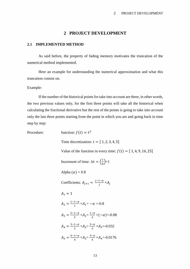
Example:
If the number of the historical points for take into account are three, in other words,
the two previous values only, for the first three points will take all the historical when
calculating the fractional derivative but the rest of the points is going to take into account
only the last three points starting from the point in which you are and going back in time
step by step:
Procedure: function: 𝑓(𝑡) = 𝑡2
Time discretization: 𝑡 = [ 1, 2, 3, 4, 5]
Value of the function in every time: 𝑓(𝑡) = [ 1, 4, 9, 16, 25]
Increment of time: Δ𝑡 = (𝑡
𝑁)=1
Alpha (𝛼) = 0.8
Coefficients: 𝐴𝑗+1 = 𝑗−1−𝛼
𝑗 ×𝐴𝑗
𝐴1 = 1
𝐴2 =1−1−𝛼
1 ×𝐴1= −𝛼 =-0.8
𝐴3 =2−1−𝛼
2 ×𝐴2=
1−𝛼
2 ×(−𝛼)=-0.08
𝐴4 =3−1−𝛼
3 ×𝐴2=
2−𝛼
3 ×𝐴3=-0.032
𝐴5 =4−1−𝛼
4 ×𝐴2=
3−𝛼
4 ×𝐴4=-0.0176

2 PROJECT DEVELOPMENT
14
The formula used:
d𝛼𝑓(𝑡)
d𝑡𝛼⋍ [(
𝑡
𝑁)−𝛼
∑ 𝐴𝑗+1𝑓 (𝑡 − 𝑗𝑡
𝑁)
𝑁−1
𝑗=0
] ( 41)
Results of the fractional derivative in every second:
Second 2: Δ𝑡−𝛼[𝐴1𝑓(𝑡) + 𝐴2𝑓(𝑡 − Δ𝑡)] =
Δ𝑡−𝛼[𝐴14 + 𝐴21] = 1−0.8[1 × 4 + (−0.8) × 1] = 3.2
Second 3: Δ𝑡−𝛼[𝐴1𝑓(𝑡) + 𝐴2𝑓(𝑡 − Δ𝑡) + 𝐴3𝑓(𝑡 − 2Δ𝑡)] =
Δ𝑡−𝛼[𝐴19 + 𝐴24 + 𝐴31]=1−0.8[1 × 9 + (−0.8) × 4 + (−0.08) × 1]= 5.72
Second 4: Δ𝑡−𝛼[𝐴1𝑓(𝑡) + 𝐴2𝑓(𝑡 − Δ𝑡) + 𝐴3𝑓(𝑡 − 2Δ𝑡) + 𝐴4𝑓(𝑡 − 3Δ𝑡)] =
Δ𝑡−𝛼[𝐴116 + 𝐴29 + 𝐴34 + 𝐴41] =
1−0.8[1 × 16 + (−0.8) × 9 + (−0.08) × 4 + (−0.032) × 1]= 8.448
Second-5: Δ𝑡−𝛼[𝐴1𝑓(𝑡) + 𝐴2𝑓(𝑡 − Δ𝑡) + 𝐴3𝑓(𝑡 − 2Δ𝑡) + 𝐴4𝑓(𝑡 − 3Δ𝑡) +
+ 𝐴5𝑓(𝑡 − 4Δ𝑡)] =
Δ𝑡−𝛼[𝐴125 + 𝐴216 + 𝐴39 + 𝐴44 + 𝐴51] =
1−0.8[1 × 25 + (−0.8) × 16 + (−0.08) × 9 + (−0.032) × 4 + (−0.0176) × 1]=
11.3344
Now with only 2 previous points of the historical:
Second 2: Δ𝑡−𝛼[𝐴1𝑓(𝑡) + 𝐴2𝑓(𝑡 − Δ𝑡)] =
Δ𝑡−𝛼[𝐴14 + 𝐴21] =1−0.8[1 × 4 + (−0.8) × 1]= 3.2
Second 3: Δ𝑡−𝛼[𝐴1𝑓(𝑡) + 𝐴2𝑓(𝑡 − Δ𝑡) + 𝐴3𝑓(𝑡 − 2Δ𝑡)] =
Δ𝑡−𝛼[𝐴19 + 𝐴24 + 𝐴31]=1−0.8[1 × 9 + (−0.8) × 4 + (−0.08) × 1]= 5.72
Second 4: Δ𝑡−𝛼[𝐴1𝑓(𝑡) + 𝐴2𝑓(𝑡 − Δ𝑡) + 𝐴3𝑓(𝑡 − 2Δ𝑡)] =
Δ𝑡−𝛼[𝐴116 + 𝐴29 + 𝐴34] =1−0.8[1 × 16 + (−0.8) × 9 + (−0.08) × 4]= 8.48

2 PROJECT DEVELOPMENT
15
Second 5: Δ𝑡−𝛼[𝐴1𝑓(𝑡) + 𝐴2𝑓(𝑡 − Δ𝑡) + 𝐴3𝑓(𝑡 − 2Δ𝑡)] =
Δ𝑡−𝛼[𝐴125 + 𝐴216 + 𝐴39] =1−0.8[1 × 25 + (−0.8) × 16 + (−0.08) × 9]= 11.48
Comparing both methods it can be said that the truncated one is less accurate and
has an increasing error in time (see fig. 1). This will be deeply studied in a concrete
situations with the Matlab program.
Figure 1: Comparison of two numerical methods made by hand.
Figure 2: Comparison of two numerical methods with Matlab program.
0
2
4
6
8
10
12
14
2 s 3 s 4 s 5 s
comparison of both numerical methods
numerical with all historical

2 PROJECT DEVELOPMENT
16
Exactly the same result has been obtained with the Matlab (fig.2). So it can be
said that the part for next different cases where the fractional derivative and the truncated
fractional derivative has been used are correct.
EMBRACING A WIDER RANGE OF CASES
With the aim of constructing a more generalist Matlab program which will be
capable to solve a wider range of different situations, another substantial implementation
has been done.
In previous year’s situation the number of points where the fractional derivate was
calculated and the final time where the same. Because of this, was not necessary to take
into account this factor of the complete formula.
(𝑡
𝑁)−𝛼
= (200
200)
−𝛼
= 1−𝛼 = 1 ( 42)
The formula implemented was:
d𝛼𝑓(𝑡)
d𝑡𝛼⋍ [∑ 𝐴𝑗+1𝑓 (𝑡 − 𝑗
𝑡
𝑁)
𝑁−1
𝑗=0
] ( 43)
In the new complete formula any vector of time can be defined.
With the purpose to prove this and ensure the good state of the Matlab program
where the fractional derivate is being tested another casuistic has been done.
Of course, it is known that for a function that is a line, its entire derivative
(alpha=1) is going to be constant with the value of the slope. In the particular case where
the function has slope one the solution of the program will be constant and with the value
one (fig.3).

2 PROJECT DEVELOPMENT
17
Figure 3: Particular case for fractional derivative.
ERRORS
In the three cases of the Matlab same study of the error between the two numerical
methods has been done. For that, the formula of the relative error applied was the
following. This error was calculated in the all historical points used (200 points):
𝑒𝑟𝑟𝑜𝑟 =[𝑓(𝑡)](𝑁) − [𝑓(𝑡)](𝑁+𝛥𝑁)
[𝑓(𝑡)](𝑁+𝛥𝑁) ( 44)
2.2 MATLAB PROGRAMES
A specific phenomenon has been chosen where a material is suffering a
deformation and its stressed has to be calculated. Of course fractional derivatives are
needed to know the stress.
The objective is to develop a generalist program which different situations of
deformation can be applied to the material chosen and take the results of the stress.
In all of them the program ask to the user how many historical points wants to
take into account and the alpha of the fractional derivative between cero and one. Between
the programs some differences rises but the main part and the way to solve numerical
results keeps being the same.

2 PROJECT DEVELOPMENT
18
2.2.1 Linear deformation imposed in time:
Function applied:
In this first case, a linear deformation in time has been done to a material (fig. 4).
With this, the stress suffered is going to be calculated with the methods named before.
Figure 4: Linear deformation input.
Analytical solution:
First, talking about the analytical formula, the most simple one was developed,
which does not need fractional derivatives to describe the stress, with other words a
punctual derivative (when alpha equals to one).
For analytical evaluation of the problem, this procedure has been followed:
The imposed displacement will be defined as 𝜀(𝑡):
𝜀(𝑡) = 𝜀𝑚(𝑡) ( 45)
The next differential equation is defined as it is a 3 parameter model (α=β=1);
𝜎(𝑡) + 𝑎d𝜎(𝑡)
d𝑡= 𝐸𝜀(𝑡) + 𝑏
d𝜀(𝑡)
d𝑡 ( 46)
This equation can be solved adding the homogenous and particular solutions, and
imposing the initial condition (in this case, the initial condition is null). Taking into
account the definition of 𝜀(𝑡) the final solution is:

2 PROJECT DEVELOPMENT
19
𝜎(𝑡) = 𝜀𝑚(𝑏 − 𝑎𝐸) (1 − 𝑒−𝑡𝑎) + 𝜀𝑚𝐸𝑡 ( 47)
The behavior curve obtained from this expression, has been compared with the
obtained from the fractional model. In this manner, is possible to compare and obtain
some conclusions about the accuracy of the designed fractional model.
Numerical solution:
With the same definition of the fractional derivative for �̇� and 𝜀̇ :
𝜎(𝑡) + 𝑎d𝜎(𝑡)
d𝑡= 𝐸𝜀(𝑡) + 𝑏
d𝜀(𝑡)
d𝑡 ( 48)
𝜎 + 𝑎�̇� = 𝐸𝜀 + 𝑏𝜀̇ ( 49)
𝜎 + 𝑎𝐷𝛼𝜎 = 𝐸𝜀 + 𝑏𝐷𝛼𝜀 ( 50)
Where the 𝐷𝛼𝜎 is going to be with the definition of fractional derivative and
taking out the first term:
d𝛼𝑓(𝑡)
d𝑡𝛼⋍ [(
𝑡
𝑁)−𝛼
∑ 𝐴𝑗+1𝑓 (𝑡 − 𝑗𝑡
𝑁)
𝑁−1
𝑗=0
] =
𝐷𝛼𝜎 ⋍ [𝛥𝑡−𝛼 (𝐴1𝜎 + ∑ 𝐴𝑗+1𝜎(𝑡 − 𝑗𝛥𝑡)
𝑁−1
𝑗=1
)] =
Introducing it in the equation 𝜎 + 𝑎𝐷𝛼𝜎 = 𝐸𝜀 + 𝑏𝐷𝛼𝜀
𝜎 + 𝑎 (𝛥𝑡−𝛼𝐴1𝜎 + 𝛥𝑡−𝛼 ∑ 𝐴𝑗+1𝜎(𝑡 − 𝑗𝛥𝑡)
𝑁−1
𝑗=1
) = 𝐸𝜀 + 𝑏𝐷𝛼𝜀
𝜎 + 𝑎𝛥𝑡−𝛼𝐴1𝜎 + 𝑎 (𝛥𝑡−𝛼 ∑ 𝐴𝑗+1𝜎(𝑡 − 𝑗𝛥𝑡)
𝑁−1
𝑗=1
) = 𝐸𝜀 + 𝑏𝐷𝛼𝜀
𝜎 + 𝑎𝛥𝑡−𝛼𝐴1𝜎 = 𝐸𝜀 + 𝑏𝐷𝛼𝜀 − 𝑎 (𝛥𝑡−𝛼 ∑ 𝐴𝑗+1𝜎(𝑡 − 𝑗𝛥𝑡)
𝑁−1
𝑗=1
)
= 𝛥𝑡−𝛼𝐴1𝜎 + 𝛥𝑡−𝛼 ∑ 𝐴𝑗+1𝜎(𝑡 − 𝑗𝛥𝑡)
𝑁−1
𝑗=1
( 51)

2 PROJECT DEVELOPMENT
20
𝜎(1 + 𝑎𝛥𝑡−𝛼𝐴1) = 𝐸𝜀 + 𝑏𝐷𝛼𝜀 − 𝑎 (𝛥𝑡−𝛼 ∑ 𝐴𝑗+1𝜎(𝑡 − 𝑗𝛥𝑡)
𝑁−1
𝑗=1
)
This is what is applied in the Matlab for the numerical resolution of the stress. As the
last formula shows fractional solving procedure is needed in stress and strain.
RESULTS
In this part of the work, different logical situations are going to be analyzed in
order to ensure that the Matlab developed runs in the appropriated way.
The first thing to prove is that for the particular case of alpha equals one, the three
curves are going to be the same (see fig. 5). As the figure 6 shows, there is no error
between them because the analytical situation for alpha one has been implemented and
selecting alpha one for the numerical make the curves be the same. Same result has been
obtained for an alpha very close to one, for alpha=0.999 (see figure 7).
Figure 5: Alpha=1 for linear input.
𝜎 =
𝐸𝜀 + 𝑏𝐷𝛼𝜀 − 𝑎 (𝛥𝑡−𝛼 ∑ 𝐴𝑗+1𝜎(𝑡 − 𝑗𝛥𝑡) 𝑁−1
𝑗=1)
(1 + 𝑎𝛥𝑡−𝛼𝐴1)
( 52)

2 PROJECT DEVELOPMENT
21
Figure 6: Error for alpha=1.
Figure 7: Alpha=0.999 for linear input.
Other interesting situation the case of alpha 1 is that no matter how many points
are taken into account in the truncated numerical method because this is the particular
case where the derivate is the classic one where only takes the previous value to solve it.
In other words, all the coefficients are going to be cero except the first one, which is going
to be one, so even taking into account less points the result is going to be the same and
the error between numerical and numerical truncated is going to be the 0.
2 PROJECT DEVELOPMENT
22
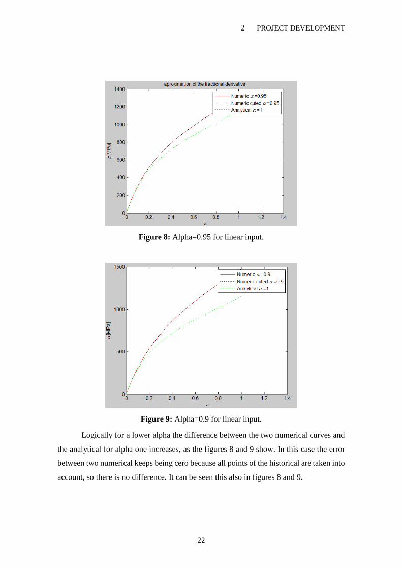
Figure 8: Alpha=0.95 for linear input.
Figure 9: Alpha=0.9 for linear input.
Logically for a lower alpha the difference between the two numerical curves and
the analytical for alpha one increases, as the figures 8 and 9 show. In this case the error
between two numerical keeps being cero because all points of the historical are taken into
account, so there is no difference. It can be seen this also in figures 8 and 9.

2 PROJECT DEVELOPMENT
23
Of course this is not going to happen with the other alpha where the error will
increase when less points are taken. Here below in figures from 10 to 13, the development
of the error for a specific alpha.
Let’s see now how the error evolves for a determinate alpha when less and less
points are taken into account. In figure 10 half of the historical is taken into account (100
points) and in figure 12 half of the half (50 points).
Figure 10: 100 points of the historical
Figure 11: Error of 100 points

2 PROJECT DEVELOPMENT
24
Figure 12: 50 points of the historical
Figure 13: error of 50 points
Now, an error exist because not taking into account all the historical (fig.11 and
13). This error will start in the point where the user has introduced in the Matlab. This is
because the way that is programed is to take all the historical until that point the user has
marked. From that point it only will take into account the last number of points selected.
Of course when less points are taken into account the error will appear sooner and will
reach higher as the figure 13 shows.

2 PROJECT DEVELOPMENT
25
It has been proved that the computational work is less when less points are used
in the definition of the fractional derivative applied.
DEEPER STUDY FOR THE ERROR
The figures from 14 to 20 show how the error evolves in any time of the test.
Different curves have been plotted depending of the number of points taking into account.
Less points will suppose a higher error as the figures. Cases of different alpha are plotted:
Figure 14: Errors for alpha=0.99 linear input
0
5
10
15
20
25
1 9
17
25
33
41
49
57
65
73
81
89
97
10
5
11
3
12
1
12
9
13
7
14
5
15
3
16
1
16
9
17
7
18
5
19
3
erro
r (%
)
Time (s)
alpha=0.99
Series1 Series2 Series3 Series4 Series5 Series6
2 PROJECT DEVELOPMENT
26
Figure 15: Errors for alpha=0.9 linear input
Figure 16: Errors for alpha=0.45 linear input
0
10
20
30
40
50
60
70
80
90
1 81
52
22
93
64
35
05
76
47
17
88
59
29
91
06
11
31
20
12
71
34
14
11
48
15
51
62
16
91
76
18
31
90
19
7
erro
r(%
)
Time(s)
alpha=0.9
0
2
4
6
8
10
12
14
16
1 8
15
22
29
36
43
50
57
64
71
78
85
92
99
10
6
11
3
12
0
12
7
13
4
14
1
14
8
15
5
16
2
16
9
17
6
18
3
19
0
19
7
erro
r(%
)
Time(s)
alpha=0.45

2 PROJECT DEVELOPMENT
27
Figure 17: Error for alpha=0.2845 linear input
Figure 18: Error for alpha=0.225 linear input
0
1
2
3
4
5
6
1 8
15
22
29
36
43
50
57
64
71
78
85
92
99
10
6
11
3
12
0
12
7
13
4
14
1
14
8
15
5
16
2
16
9
17
6
18
3
19
0
19
7
erro
r(%
)
Time(s)
alpha=0.2845
Series1 Series2 Series3 Series4 Series5 Series6
0
0,5
1
1,5
2
2,5
3
3,5
4
1 8
15
22
29
36
43
50
57
64
71
78
85
92
99
10
6
11
3
12
0
12
7
13
4
14
1
14
8
15
5
16
2
16
9
17
6
18
3
19
0
19
7
erro
r(%
)
Time(s)
alpha 0.225
Series1 Series2 Series3 Series4 Series5 Series6

2 PROJECT DEVELOPMENT
28
Figure 19: Error for alpha=0.10 linear input
Figure 20: Error for alpha=0.05 linear input
Now for a concrete number of points, for the examples of 4, 6, 8 points we are
going to see how the error changes for this the second 200 has been selected, that is the
end of the test:
0
0,2
0,4
0,6
0,8
1
1,2
1 8
15
22
29
36
43
50
57
64
71
78
85
92
99
10
6
11
3
12
0
12
7
13
4
14
1
14
8
15
5
16
2
16
9
17
6
18
3
19
0
19
7
erro
r(%
)
Time(s)
alpha=0.10
Series1 Series2 Series3 Series4 Series5 Series6
0
0,1
0,2
0,3
0,4
0,5
0,6
1 9
17
25
33
41
49
57
65
73
81
89
97
10
5
11
3
12
1
12
9
13
7
14
5
15
3
16
1
16
9
17
7
18
5
19
3
erro
r(%
)
Time(s)
alpha=0.05
Series1 Series2 Series3 Series4 Series5 Series6
2 PROJECT DEVELOPMENT
29
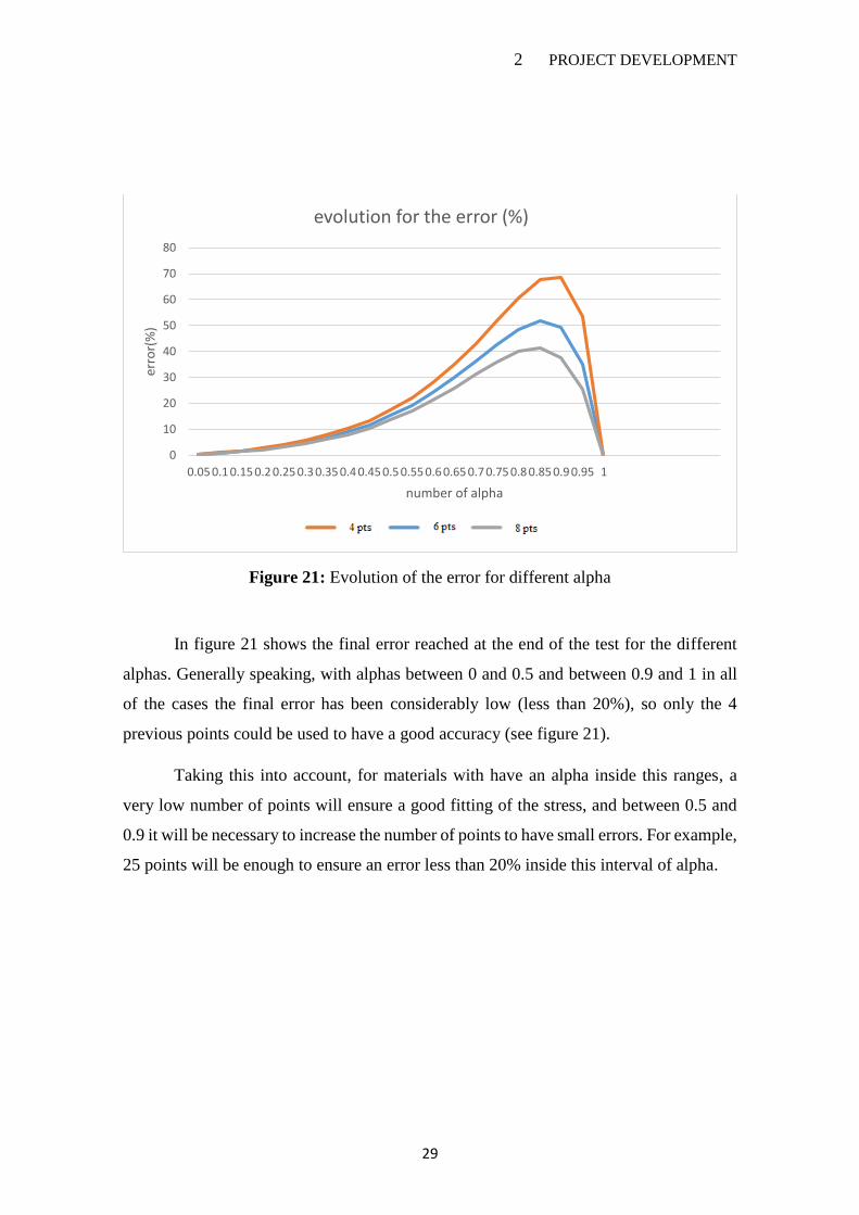
Figure 21: Evolution of the error for different alpha
In figure 21 shows the final error reached at the end of the test for the different
alphas. Generally speaking, with alphas between 0 and 0.5 and between 0.9 and 1 in all
of the cases the final error has been considerably low (less than 20%), so only the 4
previous points could be used to have a good accuracy (see figure 21).
Taking this into account, for materials with have an alpha inside this ranges, a
very low number of points will ensure a good fitting of the stress, and between 0.5 and
0.9 it will be necessary to increase the number of points to have small errors. For example,
25 points will be enough to ensure an error less than 20% inside this interval of alpha.
0
10
20
30
40
50
60
70
80
0.05 0.1 0.15 0.2 0.25 0.3 0.35 0.4 0.45 0.5 0.55 0.6 0.65 0.7 0.75 0.8 0.85 0.9 0.95 1
erro
r(%
)
number of alpha
evolution for the error (%)
6 points

2 PROJECT DEVELOPMENT
30
Figure 22: range of the curves for all the alpha
In the figure 22 it can be seen how the shape of the function change with all the
alphas from one to cero.
Now, a different input of deformation will be imposed to the same material. Some
changes will rise but the way of developing the numerical fractional derivate keeps being
the same.
2.2.2. Constant deformation imposed in time
In this second case, a constant lineal deformation in time has been done to a
material. With this, the stress suffered is going to be calculated with the methods named
before. The procedure for getting to analytical and numerical solution is going to be very
similar with some particularities explained with detail in this section.
Function applied:
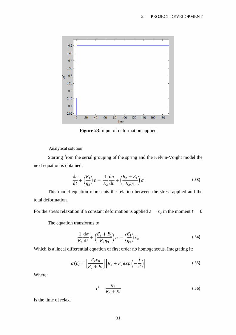
In figure 23 the graphic of the deformation applied:
2 PROJECT DEVELOPMENT
31
Figure 23: input of deformation applied
Analytical solution:
Starting from the serial grouping of the spring and the Kelvin-Voight model the
next equation is obtained:
d𝜀
d𝑡+ (
𝐸1
𝜂3) 𝜀 =
1
𝐸2
d𝜎
d𝑡+ (
𝐸2 + 𝐸1
𝐸2𝜂3) 𝜎 ( 53)
This model equation represents the relation between the stress applied and the
total deformation.
For the stress relaxation if a constant deformation is applied 𝜀 = 𝜀0 in the moment 𝑡 = 0
The equation transforms to:
1
𝐸2
d𝜎
d𝑡+ (
𝐸2 + 𝐸1
𝐸2𝜂3) 𝜎 = (
𝐸1
𝜂3) 𝜀0 ( 54)
Which is a lineal differential equation of first order no homogeneous. Integrating it:
𝜎(𝑡) = [𝐸2𝜀0
𝐸2 + 𝐸1] [𝐸1 + 𝐸2𝑒𝑥𝑝 (−
𝑡
𝜏′)] ( 55)
Where:
𝜏′ =𝜂3
𝐸2 + 𝐸1 ( 56)
Is the time of relax.

2 PROJECT DEVELOPMENT
32
This will be the equation applied in Matlab. As the equation shows, the stress is
relaxed exponentially with the time from the high initial value to the value of equilibrium.
The time of relaxation depends on the constant of the spring 𝐸2 and of the parameters of
the Kelving-Voigt 𝜂3, 𝐸1.
On the other hand, as for the example the parameters of the material are known,
𝐸1, 𝐸2, 𝜂3
Have to be determined. For that a system of equations of three equations and three
unknowns will be solved. The system will be the following:
General expression is the constitutive equation of the 3-parameter model:
𝜎 +𝜂
𝐸1 + 𝐸2
d
d𝑡𝜎 =
𝐸1𝐸2
𝐸1 + 𝐸2𝜀 + 𝜂
𝐸2
𝐸1 + 𝐸2
d
d𝑡𝜀 ( 57)
Concrete case is:
𝜎(𝑡) + 𝑎d𝛼
d𝑡𝛼𝜎 = 𝐸𝜀(𝑡) + 𝑏
d𝛼
d𝑡𝛼𝜀 ( 58)
And the identified parameters by least-square fit of Delrin𝑇𝑀in time domain where:
𝐸 = 658.2 𝑁
𝑚𝑚2
𝑎 = 32.017 𝑠𝛼
𝑏 = 120593.0𝑁
𝑚𝑚2𝑠𝛼
System:
𝑎 =𝜂3
𝐸1 + 𝐸2
𝐸 =𝐸1𝐸2
𝐸1 + 𝐸2
𝑏 = 𝜂3
𝐸2
𝐸1 + 𝐸2
Now the previous general equation can be implemented.
Numerical solution:

2 PROJECT DEVELOPMENT
33
Same resolution has been applied as before.
Results:
To ensure the good state of the program, the same situation of alpha one has been
done. The expected results are shown in this figure 24. When alpha is close to one and all
historical is taken the three curves fit:
Figure 24: Alpha=0.999 for constant input deformation
Figure 25: Alpha=0.9 for constant input deformation
2 PROJECT DEVELOPMENT
34
Figure 26: Error for all historical taken into account
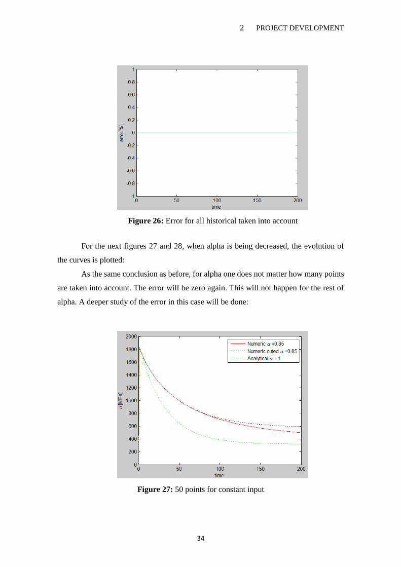
For the next figures 27 and 28, when alpha is being decreased, the evolution of
the curves is plotted:
As the same conclusion as before, for alpha one does not matter how many points
are taken into account. The error will be zero again. This will not happen for the rest of
alpha. A deeper study of the error in this case will be done:
Figure 27: 50 points for constant input

2 PROJECT DEVELOPMENT
35
Figure 28: Error for 50 points constant input
DEEPER STUDY FOR THE ERROR
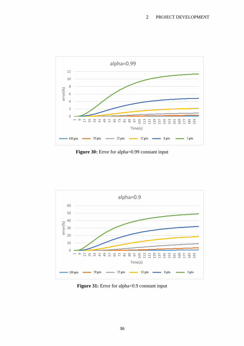
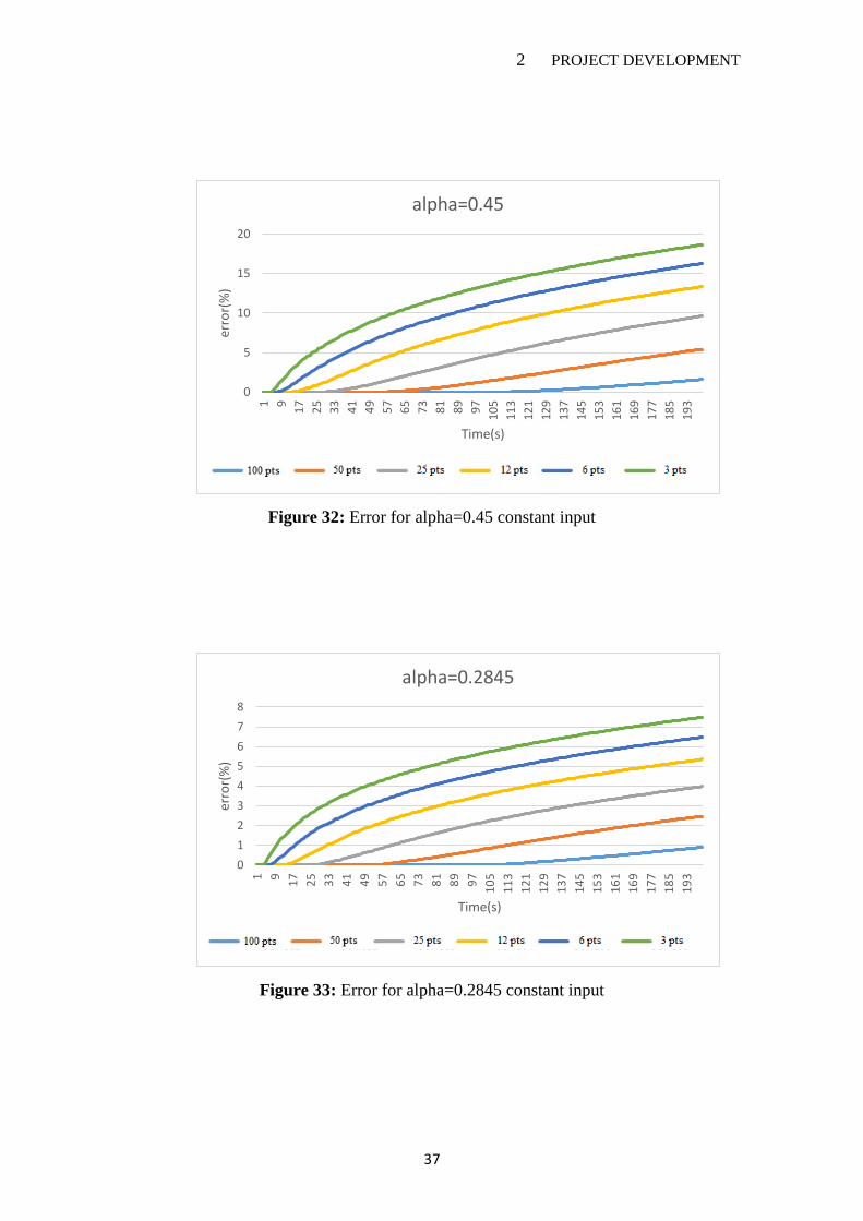
In this figures from 29 to 36, the evolution of the error for all the time instants of
the test has been obtained. This errors will be increased depending of the alpha chosen.
Other interesting point is the fact that in this case of constant deformation input,
all the errors are convergent. So even that doing a larger test the error will not increase.
More specifically speaking, for this alpha close to one, the error is very close to zero with
almost no difference on how many points are taken into account.
Figure 29: Error for alpha=0.999 constant input
0
0,2
0,4
0,6
0,8
1
1,2
1,4
1 9
17
25
33
41
49
57
65
73
81
89
97
10
5
11
3
12
1
12
9
13
7
14
5
15
3
16
1
16
9
17
7
18
5
19
3
erro
r(%
)
Time(s)
alpha=0.999
Series1 Series2 Series3 Series4 Series5 Series6
2 PROJECT DEVELOPMENT
36
Figure 30: Error for alpha=0.99 constant input
Figure 31: Error for alpha=0.9 constant input
0
2
4
6
8
10
121 9
17
25
33
41
49
57
65
73
81
89
97
10
5
11
3
12
1
12
9
13
7
14
5
15
3
16
1
16
9
17
7
18
5
19
3
erro
r(%
)
Time(s)
alpha=0.99
Series1 Series2 Series3 Series4 Series5 Series6
0
10
20
30
40
50
60
1 9
17
25
33
41
49
57
65
73
81
89
97
10
5
11
3
12
1
12
9
13
7
14
5
15
3
16
1
16
9
17
7
18
5
19
3
erro
r(%
)
Time(s)
alpha=0.9
Series1 Series2 Series3 Series4 Series5 Series6
2 PROJECT DEVELOPMENT
37
Figure 32: Error for alpha=0.45 constant input
Figure 33: Error for alpha=0.2845 constant input
0
5
10
15
20
1 9
17
25
33
41
49
57
65
73
81
89
97
10
5
11
3
12
1
12
9
13
7
14
5
15
3
16
1
16
9
17
7
18
5
19
3
erro
r(%
)
Time(s)
alpha=0.45
Series1 Series2 Series3 Series4 Series5 Series6
0
1
2
3
4
5
6
7
8
1 9
17
25
33
41
49
57
65
73
81
89
97
10
5
11
3
12
1
12
9
13
7
14
5
15
3
16
1
16
9
17
7
18
5
19
3
erro
r(%
)
Time(s)
alpha=0.2845
Series1 Series2 Series3 Series4 Series5 Series6

2 PROJECT DEVELOPMENT
38
Figure 34: Error for alpha=0.225 constant input
Figure 35: Error for alpha=0.10 for constant input
0
1
2
3
4
5
6
1 9
17
25
33
41
49
57
65
73
81
89
97
10
5
11
3
12
1
12
9
13
7
14
5
15
3
16
1
16
9
17
7
18
5
19
3
erro
r(%
)
Time(s)
alpha=0.225
Series1 Series2 Series3 Series4 Series5 Series6
0
0,2
0,4
0,6
0,8
1
1,2
1,4
1,6
1 9
17
25
33
41
49
57
65
73
81
89
97
10
5
11
3
12
1
12
9
13
7
14
5
15
3
16
1
16
9
17
7
18
5
19
3
erro
r(%
)
Time(s)
alpha=0.10
Series1 Series2 Series3 Series4 Series5 Series6

2 PROJECT DEVELOPMENT
39
Figure 36: Error for alpha=0.05 for constant input
This figure 37 show the shape of the stress functions evolution from 0 to 1.
Figure 37: Range of the curves for all the alpha
0
0,1
0,2
0,3
0,4
0,5
0,6
0,7
1 9
17
25
33
41
49
57
65
73
81
89
97
10
5
11
3
12
1
12
9
13
7
14
5
15
3
16
1
16
9
17
7
18
5
19
3
erro
r(%
)
Time(s)
alpha=0.05
Series1 Series2 Series3 Series4 Series5 Series6

2 PROJECT DEVELOPMENT
40
Figure 38: Evolution of the error for different alpha
In figure 38 shows the final error reached at the end of the test for the different
alphas.
Generally speaking, with alphas between 0 and 0.5 and between 0.9 and 1 in all
of the cases the final error has been considerably low(less than 20%), so only the 4
previous points can be used (see figure 38).
Taking this into account, for materials with have an alpha inside this ranges a very
low number of points will ensure a good fitting of the stress, and between 0.5 and 0.9 it
will be necessary to increase the number of points to have small errors. For example, 25
points will be enough to ensure an error less than 20% inside this interval of alpha.
0
10
20
30
40
50
60
0.050.10.150.20.250.30.350.40.450.50.550.60.650.70.750.80.850.90.95 1
erro
r(%
)
number of alpha
evolution for the error (%)
6 points
3 OTHER OPTIONS OF HISTORICAL TRUNCATION
41
3 OTHER OPTIONS OF HISTORICAL TRUNCATION
There are more ways to truncate in the historical. From the methods to calculate
de fractional derivative the first one has been applied.
Here graphically the difference between the two methods:
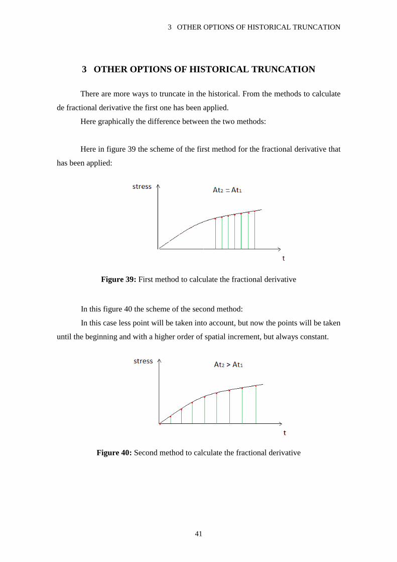
Here in figure 39 the scheme of the first method for the fractional derivative that
has been applied:
Figure 39: First method to calculate the fractional derivative
In this figure 40 the scheme of the second method:
In this case less point will be taken into account, but now the points will be taken
until the beginning and with a higher order of spatial increment, but always constant.
Figure 40: Second method to calculate the fractional derivative
2 PROJECT DEVELOPMENT
42
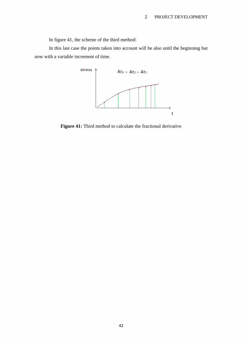
In figure 41, the scheme of the third method:
In this last case the points taken into account will be also until the beginning but
now with a variable increment of time.
Figure 41: Third method to calculate the fractional derivative

4 CONCLUSIONS AND FUTURE LINES OF RESEARCH
43
4 CONCLUSIONS AND FUTURE LINES OF RESEARCH
Conclusions
The main objective of developing an algorithm which does not take into account
the all historical has been completed.
Previously 200 points were required, and after applying this method only 4 and
25. This will suppose an important decrease of the computational effort.
For the cases studied, 4 points will be enough to describe the process with a good
accuracy in intervals, [0, 0.5) and (0.95, 1] and 25 for the interval [0.5, 0.95] ensuring an
error less than 20% in all cases.
For future lines of research
Analytical solutions for a different alpha could be implemented to show how it
fits with the numerical with the all historical when alpha different to one.
Other cutting methods could be implemented and compared between them and
with the one explained in this project to see which will be the best.
This method could be applied to the hysteretic behavior.
Implement the selected method in a FEM program.
4.1 CONTRIBUTIONS, WHICH IN LEARNING, THE PROJECT HAVE LED
Academically, this project provides a deep knowledge in numerical methods and
fractional derivatives. During this project the real application of numerical methods can
be seen.

2 PROJECT DEVELOPMENT
44
How fractional derivatives works and which are the most used expressions of them
nowadays. Apart from that, how they are applied to rheological or viscoelastic models
and how they improve the response when working with the curve fitting.
How a composite or any other material is defined by using numerical methods and
fractional derivatives has been understood.
How useful the rheological models are for simulating the behavior of any material
are has been learnt.
It has been learnt how to manage for developing a large project like this that treats
a totally new topic. For that, working in an environment like this requires a big personal
effort for bringing the project forward.
Programing skills have been improved gaining more confidence and security on
it.
Having lived in another country and learning a new language made this experience
even more interesting.
The complexity of the project such as living alone in a new country has done a
good improvement in the responsibilities and organization of the diary lifestyle.
4.2 NEW PRODUCTS, BUSINESS UNITS OR DEVELOPMENTS THAT MAY
ARISE FROM THE MASTER PROJECT
Nowadays, Finite Element programs are really used in every sector of industrial
manufacturing and investigation. Planes, cars and any type of products must be tested to
ensure their capability of facing strong external conditions or daily use. Any product
development requires a large testing process and when working with certain materials as
composite materials, metals or plastics finite tests without risking a lot of money.

2 PROJECT DEVELOPMENT
45
Until recently, composite material where used in a really specific and high
qualified industrial activities as aeronautic, but nowadays, composite materials are being
introduced inside the general product market bit by bit. This opens lots of possibilities to
the different manufacturers, and an investment in finite element programs will be soon
required by these types of enterprises. Lots of these enterprises will require a personalized
Finite Element program which works with a specific behavior law and is there, where this
project really takes its place. As said, composite materials are the material of the future
so the market will grow.
In the development field it has to be said that still today is a lot to do. New and
better ways of implementing Fractional derivatives are being studied and the aim is to
control this topic as much as possible.

5 REFERENCES
46
5 REFERENCES
1. Leibniz, G., Leibnizsche Mathematische Schriften, Georg Olm Verlag, Hildesheim,
1962. 2. Lacroix, S., Traité du calcul differentiel et du calcul intégral, Courcier, Paris, 1819.
3. Abel, N., ‘Solution de quelques problèmes à l’aide d’intégrales définites’,
Christiania Grondahl, Norway, 1881, pp. 16–18.
4. Liouville, J., ‘Mémoire sur le calcul des différentielles à indices quelconques’,
Journal d’Ecole Polytechnique 13, 1832, 71–162.
5. Liouville, J., ‘Mémoire sur quelques quéstions de géomerie et de mécanique,
et sur un nouveau genre de calcul pour résoudre ces quéstions’, Journal
d’Ecole Polytechnique 13, 1832, 1–69.
6. Liouville, J., ‘Mémoire sur le théoreme des fonctions complémentaires’, Journal
für die reine und angewandte Mathematik 11, 1834, 1–19
7. Ross, B., ‘A brief history and exposition of the fundamental theory of
fractional calculus’, Fractional Calculus and Its Applications, Lecture Notes
in Mathematics, Vol. 457, Springer-Verlag, Berlin, 1975.
8. Nutting, P. G., ‘A new general law of deformation’, Journal of the Franklin Institute
191, 1921, 679–685
9. Gemant, A., ‘A method of analyzing experimental results obtained from elasto-viscous
bodies’, Physics 7, 1936, 311–317. 10. Gemant, A., ‘On fractional differentials’, The Philosophical Magazine 25, 1938, 540–
549.
11. Scott Blair, G. W. and Caffyn, J. E., ‘An application of the theory of quasi-properties to
the treatment of anomalous strain-stress relations’, The Philosophical Magazine 40,
1949, 80–94.
12. Caputo, M., ‘Vibrations on an infinite viscoelastic layer with a dissipative memory’,
Journal of the Acoustical Society of America 56(3), 1974, 897–904.
13. Caputo, M. and Mainardi, F., ‘A new dissipation model based on memory mechanism’,
Pure and Applied Geophysics 91, 1971, 134–147.
14. Bagley, R. L. and Torvik, P. J., ‘A theoretical basis for the application of fractional
calculus to viscoelasticity’, Journal of Rheology 27(3), 1983, 201–210.
15. Bagley, R. L. and Torvik, P. J., ‘On the fractional calculus model of viscoelastic
behaviour’, Journal of Rheology 30(1), 1986, 133–155.
16. Padovan, J., ‘Computational algorithms for FE formulations involving fractional
operators’, Computational Mechanics 2, 1987, 271–287.
17. Koeller, R. C., ‘Applications of fractional calculus to the theory of viscoelasticity’,
ASME Journal of Applied Mechanics 51, 1984, 299–307.
18. Enelund, M. and Josefson, B. M., ‘Time-domain Finite Element analysis of viscoelastic
structures with fractional derivatives constitutive relations’, AIAA Journal 35(10),
1997, 1630–1637.

2 PROJECT DEVELOPMENT
47
19. Enelund M., Mähler, L., Runesson, B., and Josefson, B. M., ‘Formulation and
integration of the standard linear viscoelastic solid with fractional order rate laws’,
Journal of Solids and Structures 36, 1999, 2417–2442.
20. Gaul, L. and Schanz, M., ‘A comparative study of three boundary element approaches
to calculate the transient response of viscoelastic solids with unbounded domains’,
Computer Methods in Applied Mechanics and Engineering 179, 1999, 111–123.
21. Gaul, L., ‘The influence of damping on waves and vibrations’, Mechanical Systems
and Signal Processing 13(1), 1999, 1–30.
22. Podlubny, I., Fractional Differential Equations, Academic Press, San Diego, CA,
1999.
23. Grünwald, A. K., ‘Über ’begrenzte‘ Derivationen und deren Anwendung’, Zeitschrift
für angewandte Mathematik und Physik 12, 1867, 441–480.
24. Oldham, K. B. and Spanier, J., The Fractional Calculus, Academic Press, New York,
1974
25. S. Marguet, P. Rozycki, and L. Gornet. A rate dependent constitutive model for
carbon fiber reinforced plastic woven fabrics. Mechanics of Advanced
Materials and Structures, 14:619–631, 2007.
26. A.F. Johnson, A.K. Pickett, and P. Rozycki. Computational methods for
predicting impact damage in composites structures. Composites Science
and Technology, 61:2183–2192, 2001.
27. M. Mateos, L. Gornet, and P. Rozycki. Comportement hystérétique en
cisaillement des composites renforcés des fibres. In Comptes Rendus des JNC
18, 2013.
28. M. Rabius, R.K. Kapania, R.D. Mo_t, M. Mishra, and N. Goulbourne. A
modified fractional calculus approach to model hysteresis. Journal of
Applied Mechanics, 77:0310041-0310048, 2010.
29. M. Mateos, L. Gornet, P. Rozycki, L. Aretxabaleta. Hysteretic shear
behavior of Fibre-Reinforced composite laminates. EUROPEAN
CONFERENCE ON COMPOSITE MATERIALS, Seville, Spain, 22-26 June
2014
30. André Schmidt, Lothar Gaul. Finite Element Formulation of Viscoelastic
Constitutive Equations Using Fractional Time Derivatives. 2002 Kluwer
Academic Publishers.
31. Schmidt, A., Lotsch, M., Gaul, L. Implementation of a new method
for the computation of fractionally damped structures into discretization
methos. Institute of Applied and Experimental Mechanics.
32. Dr. Pedro Arafet Padilla, MSc. Hugo Domínguez Abreu, Dr. Francisco
Chang Mumañ. Una introducción al cálculo fraccionario. Facultad de
Ing. Eléctrica Universidad de Oriente, Mayo 2008.

2 PROJECT DEVELOPMENT
48
33. Andre´ Schmidt, Lothar Gaul. On the numerical evaluation of fractional
derivatives in multi-degree-of-freedom systems. Institut für Angewandte
und Experimentelle Mechanik, Universität Stuttgart 2005.
34. J.Padovan. computational algorithms for FE formulations involving
fractional operators. The university of Akron, USA 1987
35. Richard L. Magin. Fractional calculus in bioengineering (chapter VII).
BH 2006
36. Modesto Mateos. Fundamentals and Plasticity chapters of Master class notes
from Mondragon University.
37. Mikel Ezkurra. Numerical methods in Mechanical Engineering. Master class
notes from Mondragon University.
38. Mikel Alzuguren. Viscous and damage effects modelling for polymeric and
composite materials by fractional models: finite element implementation.Final
master project from Mondragon University 2014.
39. Comportamiento reológico de los polímeros. Viscoelasticidad. Oviedo
University
Top Related