


Idiomas
Páginas
Jurídico


December 23, 2019
1
Individual head models for estimating the 1
TMS-induced electric field in rat brain 2
Lari M. Koponen1,*, Matti Stenroos1, Jaakko O. Nieminen1, Kimmo Jokivarsi2, Olli Gröhn2, Risto J. 3
Ilmoniemi1 4
1Department of Neuroscience and Biomedical Engineering, Aalto University School of Science, Espoo, 5
Finland 6
2A.I. Virtanen Institute, University of Eastern Finland, Kuopio, Finland 7
*Correspondence to [email protected] 8
Abstract 9
In transcranial magnetic stimulation (TMS), the initial cortical activation due to stimulation is 10
determined by the state of the brain and the magnitude, waveform, and direction of the induced 11
electric field (E-field) in the cortex. The E-field distribution depends on the conductivity geometry of 12
the head. The effects of deviations from a spherically symmetric conductivity profile have been 13
studied in detail in humans. In small mammals, such as rats, these effects are more pronounced due 14
to their smaller and less spherical heads. In this study, we describe a simple method for building 15
individual realistically shaped head models for rats from high-resolution X-ray tomography images. 16
We computed the TMS-induced E-field with the boundary element method and assessed the effect 17
of head-model simplifications on the estimated E-field. The deviations from spherical symmetry have 18
large, non-trivial effects on the E-field distribution: in some cases, even the direction of the E-field in 19
the cortex cannot be reliably predicted by the coil orientation unless these deviations are properly 20
considered. 21
author/funder. All rights reserved. No reuse allowed without permission. The copyright holder for this preprint (which was not peer-reviewed) is the. https://doi.org/10.1101/2019.12.23.886861doi: bioRxiv preprint
December 23, 2019
2
Introduction 22
In transcranial magnetic stimulation (TMS), a pulsed magnetic field induces an electric field (E-field) 23
in the brain, causing action potentials in the targeted cortical region. In a typical TMS pulse, the 24
magnetic field is increased from 0 to 1–2 tesla in less than 100 µs, which induces an E-field of the 25
order of 100 V/m. TMS has established clinical applications in, e.g., presurgical mapping of brain 26
functions1–4 and treatment of drug-resistant major depression5–7. Promising clinical applications are 27
emerging, such as stroke rehabilitation8–10 and treatment of chronic pain11,12. 28
The TMS-induced E-field accumulates charge at cell membranes, causing their local de- or 29
hyperpolarisation13. This can happen in several ways: The E-field gradient polarises long straight 30
sections of an axon, the E-field polarises terminations and sharp turns of an axon, or a discontinuity 31
in the E-field due to different tissue properties polarises an axon passing through the tissue 32
interface. The last two are likely the strongest mechanisms14. In all three cases, the polarisation 33
depends on the direction of the induced E-field and is proportional to its magnitude14. 34
Optimal interpretation of data obtained by combining TMS with functional brain imaging requires 35
knowledge of the induced E-field distribution. For example, different E-field orientations even in the 36
same target location recruit different neuronal populations15. Computing the E-field requires a 37
model of the electrical conductivity distribution of the head, often in the form of a volume 38
conductor model (VCM). Sometimes a simple VCM is entirely adequate: For example, for human 39
TMS with the coil near the vertex, the location of the resulting E-field maximum can be computed 40
quite accurately with a spherically symmetric VCM fitted to the local radius of curvature16. However, 41
even for human TMS, such a spherical model can be inadequate when stimulating the frontal or 42
occipital lobes: The E-field-magnitude prediction can be off by tens of percent—even when only 43
considering the error relative to the E-field-magnitude prediction in the motor cortex, i.e., the 44
prediction error relevant to a typical experiment where the desired stimulation intensity is 45
author/funder. All rights reserved. No reuse allowed without permission. The copyright holder for this preprint (which was not peer-reviewed) is the. https://doi.org/10.1101/2019.12.23.886861doi: bioRxiv preprint
December 23, 2019
3
proportional to individual motor threshold16. For rodent TMS, the required level of detail in the VCM 46
has not been studied. 47
There is increasing interest to use TMS in rodents due to a myriad of genetically modified animals 48
and disease models available. As more invasive recording techniques can be used in rodents than in 49
humans, and as brain tissue is available for histological and molecular analysis, rodent TMS studies 50
are valuable, e.g., in studying brain plasticity caused by repetitive TMS17 and TMS-induced disease 51
modification18. Rodent studies allow also assessing, e.g., gene expression following repetitive 52
TMS19,20. In previous experimental TMS studies involving rats, the head has been approximated with 53
a body-shaped volume of uniform conductivity21, with concentric ellipsoids22, or with a spherical 54
model23. In addition, the infinite homogeneous conductor model has been used24; for a rat, the latter 55
model overestimates the induced E-field by a factor between five and eight25 as it fails to capture the 56
reduction in stimulation efficiency for coils much larger than the head26 . In such cases of not having 57
a finite VCM and overall in cases, where a VCM is not used, the TMS experimenters often target the 58
stimulation using a line-of-sight model (this is called line navigation), in which the E-field maximum is 59
assumed to be directly below the coil centre and E-field orientation is assumed to correspond to coil 60
orientation24. For humans, subject-specific head models are derived from magnetic resonance 61
images using pipelines that combine various pieces of software, such as FreeSurfer27, FSL28, and 62
SPM29. For the rat head, we are not aware of any proposed recipe for combining software algorithms 63
to create subject-specific realistic head models. Rather, modelling studies often use post-mortem 64
anatomical atlas data for their animal models26,30. 65
Here, we describe a simple processing pipeline for generating individual head models from micro-66
scale computed tomography (µCT) data and computing the E-field using reciprocity and the 67
boundary element method (BEM). With the resulting efficient procedure, we computed TMS-68
induced E-fields in a rat head using VCMs with varying level of detail. We compare four levels of 69
detail: line navigation, a spherically symmetric head model fitted to the inner skull surface, a 70
author/funder. All rights reserved. No reuse allowed without permission. The copyright holder for this preprint (which was not peer-reviewed) is the. https://doi.org/10.1101/2019.12.23.886861doi: bioRxiv preprint

December 23, 2019
4
realistically shaped single-compartment (1C) model that follows the body outline of the rat similarly 71
to the model used by Salvador and Miranda21, and two-compartment (2C) models that contain the 72
body outline and the skull. As a reference model, we use a high-density model which further 73
includes the spine and eyes. 74
Results 75
We built five different head models for one adult male Wistar rat—a spherical model, a 1C model, 76
two 2C models (with and without spine, respectively), and a high-resolution reference 3C model 77
(with the spine and eyes)—and computed the TMS-induced E-field for 35 different coil positions 78
shown in Fig. 1. These positions span a 10 mm × 15 mm region on the scalp, covering the superior 79
parts of the cortex. For each position, we studied all tangential coil orientations with a 10° step size, 80
resulting in 630 unique coil placements. Compared to the reference model, the cortical E-field in the 81
2C model with spine had a relative error (RE) of 7.6±1.6% over all coil positions and orientations 82
(mean ± standard deviation) and 4.7±2.4% in the region of the strongest fields (i.e., where the E-field 83
energy density exceeded 50% of its maximum, see Methods); omitting the spine, the error increased 84
to 9.6±2.4% (5.1±2.2% in the region of the strongest fields). Both of these errors were, however, far 85
smaller than the errors arising from omitting the skull: the 1C model had an RE of 64±10% 86
(41.1±4.6% in the region of the strongest fields), making it worse than the spherical model (RE 87
45.0±2.5%, and 35.2±7.0% in the region of the strongest fields). The RE is sensitive to all types of 88
errors in the E-field prediction, including its overall magnitude. Errors in the overall magnitude, 89
however, have a limited effect on typical TMS experiments, where the stimulation intensity is 90
normalised to an experimentally determined motor threshold. Omitting the general magnitude, the 91
correlation errors (CCE) of the E-field patterns were 0.53±0.23%, 0.73±0.33%, 16.2±2.9%, and 92
17.5±2.8%, respectively. For the region of the strongest fields, the correlation errors increased to 93
0.9±1.0%, 1.1±1.3%, 54±25%, and 35±25%, respectively. Further omitting even local magnitudes, the 94
mean angular errors in the direction of the cortical E-field were 3.5±0.6°, 4.6±0.9°, 26.8±4.6°, and 95
author/funder. All rights reserved. No reuse allowed without permission. The copyright holder for this preprint (which was not peer-reviewed) is the. https://doi.org/10.1101/2019.12.23.886861doi: bioRxiv preprint

December 23, 2019
5
25.1±1.8°, respectively. For the region of the strongest fields, the mean angular errors were reduced 96
to 1.6±1.2°, 1.5±1.0°, 10.8±4.4°, and 13.7±3.6°, respectively. As the difference between the two 2C 97
models in the region of strongest fields was relatively small with all these measures, we will for 98
clarity omit the 2C model with spine from Fig. 2. 99
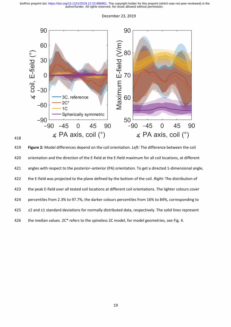
In realistic head geometry, the E-field magnitude depended on the coil orientation. Starting from the 100
posterior–anterior (PA) orientation shown in Fig. 1, the peak E-field magnitude first increased when 101
the coil was rotated to either direction, but then dropped sharply when the coil was close to ±90° 102
from the PA direction (Fig. 2). Because of this behaviour, the E-field orientation near the E-field 103
maximum was closer to the PA direction than could be expected from the coil orientation. That is, in 104
the left panel of Fig. 2, the direction of the error has opposite sign to the coil orientation. With both 105
the reference model and the 2C models, the error increased until an angle of about ±70°, at which 106
point the discrepancy between the coil and the E-field direction varied between –10 and 70° 107
depending on the coil location. The 1C model captured only a fraction of this effect; in the 1C model 108
the stimulation direction was on average closer to the PA direction than could be expected from the 109
coil orientation, but the difference was only a few degrees instead of up to several tens of degrees. 110
In the spherically symmetric model, the median orientation error over all locations was close to zero. 111
There was, however, a coil-location-dependent orientation error, which resulted from the coil 112
locations following the surface of the scalp and not that of the spherical geometry. The orientation-113
dependence of the field magnitude was likely due to the oblong shape of the rat head and the 114
cranial compartment, as almost no such drop occurred in the spherical model. 115
Defining the true stimulation target as the location of the maximum of the induced E-field in the 116
cortex in the realistic head geometry, the true target was systematically more posterior and medial 117
than expected from line navigation, the spherical head model, or the 1C head model. The error 118
depended on the coil orientation and location. The median error for line navigation was 7.3 mm (for 119
5% of the coil placements the error was greater than 12.7 mm); for the spherical head model and 120
author/funder. All rights reserved. No reuse allowed without permission. The copyright holder for this preprint (which was not peer-reviewed) is the. https://doi.org/10.1101/2019.12.23.886861doi: bioRxiv preprint

December 23, 2019
6
the 1C model, the errors were 6.3 mm (95%: 12.2 mm) and 7.2 mm (95%: 12.0 mm), respectively; 121
whereas the 2C models with and without spine had median errors of just 0.3 mm (95%: 6.0 mm) and 122
0.4 mm (95%: 7.2 mm), respectively. A cross comparison of the prediction differences between the 123
models is shown in Fig. 3. Line navigation, the spherical head model, and the 1C head model 124
produced similar, similarly incorrect, predictions. The large systematic errors in the predicted 125
stimulation location highlight the importance of an adequate model. In addition to the systematic 126
errors, the data underlying Figs. 2 and 3 contain further several coil-placement-dependent outliers 127
that could not be predicted without modelling the skull. These largest prediction errors occurred 128
when either the coil orientation was close to the PA orientation and the true stimulation maximum 129
was in the brainstem, as seen in, e.g., Fig. 4, or the coil orientation was such that a large part of the 130
windings passed directly above either eye of the rat and the true stimulation maximum was close to 131
the hole in the skull behind that eye irrespective of the actual coil position. In the first case, the E-132
field maximum corresponded to the location in which the brainstem passes through the back of the 133
skull. That is, a larger proportion of the induced currents flowed through the path of least resistance, 134
and consequently an E-field maximum arose in the proximity of the hole in the skull. In the second 135
case, a similar phenomenon occurred with the hole behind the eye. 136
Discussion 137
We described a simple method for producing subject-specific realistic-head-geometry BEM models 138
for computing the TMS-induced E-field in small rodents. Compared to line navigation, a subject-139
specific realistic model allows better estimation of the location and extent of the stimulation. 140
Compared to even a subject-specific spherical model, the realistic model further allows better 141
estimation of the stimulation dose. In addition, we demonstrated that the features of the skull 142
geometry—especially the holes in the skull—have a large effect on the E-field distribution. As the 143
described method can model these holes in the skull, it can accurately model two most influential 144
parts of the head geometry, the head shape and the skull surface in small rodents and other animals 145
author/funder. All rights reserved. No reuse allowed without permission. The copyright holder for this preprint (which was not peer-reviewed) is the. https://doi.org/10.1101/2019.12.23.886861doi: bioRxiv preprint
December 23, 2019
7
with relatively large holes in their skulls. Due to the difficult extraction of soft-tissue boundaries 146
from X-ray tomography images, the differences between different soft tissues were not modelled. 147
We compared our 2C model with previously used simpler ones and demonstrated that both the 1C 148
model of the rat and the spherical approximation of its skull failed to capture the characteristic 149
behaviour of the TMS-induced E-field in the rat brain. Further, the spherical approximation caused a 150
much larger error in the E-field calculation in the rat than what had previously been observed in 151
humans16. This is most likely due to a combination of two things: a less spherical head shape and, 152
relative to the head, a much larger coil in rat TMS. In realistic head geometry, the E-field maximum is 153
generally not directly below the coil and the peak amplitude of the E-field depends strongly on the 154
coil orientation. The 1C model manages to capture some of these effects, qualitatively, but 155
underestimates their strength and is unable to see the E-field focusing caused by holes in the skull. 156
As this focusing effect seems to cause the largest differences between the models, the next logical 157
improvement to our 2C head model would be adding more detail to these regions (such as the eyes 158
in the reference model). Another possibility is to add further tissue compartments spanning through 159
the holes in the skull (which would be the case with cerebrospinal fluid), with, for example, a BEM 160
solver that supports the use of junctioned geometry31. 161
The main source for numerical uncertainty in surface-based models arises from the discretisation of 162
the modelled surfaces. We observed only a small difference (correlation error about 1%) due to 163
halving the mesh density of the head model. In addition, the coil model resolution had only a small 164
effect: To test that the coil model was sufficiently accurate, we substituted our high-resolution coil 165
model with a simplified low-resolution model, which also assumed the 9-mm-tall windings thin. This 166
underestimated the E-field by 3% in all volume conductor models, but produced otherwise 167
essentially indistinguishable distributions with, e.g., less than 0.5° angular error in each model. 168
author/funder. All rights reserved. No reuse allowed without permission. The copyright holder for this preprint (which was not peer-reviewed) is the. https://doi.org/10.1101/2019.12.23.886861doi: bioRxiv preprint

December 23, 2019
8
Conclusion 169
The small and far-from-spherical head of the rat emphasises the effects of conductivity boundaries 170
on TMS-induced E-field distributions compared to those seen in the human head. Correct 171
determination of the stimulus location and orientation requires considering these effects, when TMS 172
experiments with small animals are designed. 173
Acknowledgements 174
This research was supported by the Finnish Cultural Foundation, the Jane and Aatos Erkko 175
Foundation, and the Academy of Finland (Decisions No. 255347, 265680, 283105, and 294625). 176
Methods 177
Head model generation 178
In a realistically shaped magnetoencephalography (MEG) or TMS forward model, the inner-skull 179
surface has the largest impact on the volume current flow. To accurately represent this surface, we 180
built a model based on a high-resolution X-ray tomography data (Flex CT, GMI, Northridge, CA, USA) 181
of the head of a male Wistar rat (weight 617 g). The animal imaging procedures were approved by 182
the University of Eastern Finland animal care committee and performed in accordance with their 183
regulations and with the guidelines of the European Community Council Directives 2010/63/EU. The 184
imaging was done using isotropic 0.17-mm voxels (cone beam acquisition, 256 projections, 2-by-2 185
binning, 512 × 512 × 512 image matrix, 60 kVp tube voltage, 450 μA tube current). The surface 186
meshes that represent conductivity boundaries were extracted by segmenting the image into air, 187
body, and bone. The imaging modality provided good contrast between these three, allowing simple 188
but robust segmentation: We set thresholds halfway between the two main peaks in the intensity 189
histogram (air and sum of all soft tissues, respectively; with our threshold at approximately –500 190
Hounsfield units (HU)) and after the end of the soft-tissue peak at approximately 500 HU. The 191
author/funder. All rights reserved. No reuse allowed without permission. The copyright holder for this preprint (which was not peer-reviewed) is the. https://doi.org/10.1101/2019.12.23.886861doi: bioRxiv preprint
December 23, 2019
9
segmented body was smoothed by computing its morphological closure with a 2-mm-radius 192
spherical kernel (in addition to smoothing the surface, this operation filled small channels in the 193
nose and ears, considerably reducing the number of vertices needed to model the body outline), and 194
the skull was smoothed similarly with a 1-mm-radius spherical kernel. Finally, two boundary surfaces 195
were extracted from volumetric tetrahedral meshes generated with “vol2mesh” function (iso2mesh, 196
iso2mesh.sourceforge.net)32. The resulting high-resolution meshes for the reference model are 197
shown in Fig. 1. The body mesh consists of 13037 vertices and 26070 faces (average edge length 198
0.95 mm, with a standard deviation of 0.12 mm), and the skull–spine mesh consists of 24318 199
vertices and 48804 faces, with an average edge length of 0.54 mm (standard deviation 0.12 mm). As 200
the rat skull contains several large holes anterior, posterior, and inferior to the brain volume, one 201
cannot model it using closed inner- and outer-skull surfaces as is conveniently done with human 202
skulls. This poses a problem, as common meshing tools and BEM solvers assume that each boundary 203
surface is closed and that the conductivity contrast across each boundary is constant. We overcame 204
this problem by requiring that the intracranial and body conductivities are equal—a common 205
assumption in conductivity parameters also in human studies. Then, we connected the inner- and 206
outermost volumes which allowed interpreting the three-compartment model as a two-207
compartment (2C) model where we have one closed skull surface (with at least one hole) floating 208
inside the body surface. With this approach, we lose the ability to simply have different conductivity 209
values for the intracranial volume and the rest of the body but gain the ability to easily model any 210
number of holes in the skull. From computational point of view, further conductivity details can be 211
added by adding further geometric entities inside the body surface: For the reference model, we 212
added the eyes, which could also be extracted from the µCT data. Unlike with the obvious high-213
contrast interfaces from air to body and from body to skull, the process for extracting the eyes could 214
not be automated, as the signal-to-noise ratio between the eyes and their surroundings was far 215
below 1. We localized the eyes from a 3-dimensional visualization of the body surface, surrounded 216
them with 8.33-mm cubic bounding boxes, and extracted them from their respective bounding 217
author/funder. All rights reserved. No reuse allowed without permission. The copyright holder for this preprint (which was not peer-reviewed) is the. https://doi.org/10.1101/2019.12.23.886861doi: bioRxiv preprint

December 23, 2019
10
boxes by applying median filtering (7 × 7 × 7 kernel, effective resolution 1.2 mm), and compensated 218
for the slight field inhomogeneity in the µCT data by manually selecting separate isolevels to extract 219
either eye. The mesh for eyes has 479 vertices and 950 elements, which brought the total vertex 220
count for the reference model to 37834 and the total element count to 75824. For the 2C model, the 221
skull–spine was independently meshed with a mean edge length of 0.67 mm, resulting in 15238 222
vertices and 30636 elements. The spineless skull was meshed with the same resolution, which 223
resulted in 12426 vertices and 24964 elements. Finally, the two 2C models and the 1C model used a 224
body mesh with a mean edge length of 1.4 mm (5924 vertices and 11844 elements). 225
The extent of the brain inside the intracranial cavity was estimated visually, and the corresponding 226
volume was filled with manual voxel painting with GNU Image Manipulation Program 227
(www.gimp.org). The E-field was computed on a surface spanned in the outermost part of this brain 228
volume, at the depth of at least 1 mm from the skull. This distance was chosen to ensure the 229
numerical stability of the solver. The surface estimation was done using a volumetric mask (i.e., 230
subtracting a 1-mm dilated skull mask from the brain mask) and then triangulating the boundary of 231
this modified brain volume. 232
Spherically symmetric head model 233
There is a relatively large region of hole-free skull above the centre of the rat head, where we fitted 234
a sphere based on the local inner-skull surface; the centre of the fitted sphere (origin) was 14.4 mm 235
from the local inner-skull surface (Fig. 4), the maximum distance from the cortex to the origin being 236
15.5 mm. The shortest distance between the scalp at the coil locations and the origin was 15.4 mm. 237
We could thus fit a sphere that was fully between the brain volume and the nearest part of coil 238
windings, meaning that the E-field in the whole brain could be computed using this spherical model 239
(although the spherical head model does not depend on the radial conductivity profile and thus on 240
the head size, the model is only valid for sources at radii smaller than the smallest distance from the 241
origin to the coil33). 242
author/funder. All rights reserved. No reuse allowed without permission. The copyright holder for this preprint (which was not peer-reviewed) is the. https://doi.org/10.1101/2019.12.23.886861doi: bioRxiv preprint

December 23, 2019
11
We needed to calculate the induced E-field everywhere in the cortex for different coil positions and, 243
ideally, would have liked to fit local spheres for all those positions. The shape of the rat head made 244
this re-fitting problematic, as, for most non-central positions, the “other end” of the brain would no 245
longer have been inside such a sphere, and the model would have been both physically invalid and 246
mathematically wrong for those remote regions. Here we overcame this problem by interpreting the 247
centrally fitted sphere as the global spherical approximation of the head, as it nicely covered the 248
whole brain, and was in size similar to, e.g., the spherical model used in23. We computed the E-field 249
in the spherical model with the analytical closed-form solution33. 250
Boundary element method 251
The TMS forward problem being reciprocal to the MEG forward problem34, the TMS-induced E-field 252
can be obtained by computing the MEG forward problem with the TMS-coil as the pick-up coil35. The 253
boundary element method is increasingly popular for solving this MEG forward problem. BEM is 254
tailored for problems where the geometry can be described by a few piecewise homogeneous 255
isotropic regions, such as the brain, cerebrospinal fluid, skull, and scalp (or in our case, mean body 256
tissue). Key benefits of using a BEM instead of a finite element model or some other volume-based 257
model are its lower memory and computation-time requirement and the ease of segmentation, 258
meshing and visualisation, as only the extracted conductivity boundaries need to be meshed and 259
discretisation is performed only on these boundary surfaces. Consequently, a typical high-resolution 260
3S model consists of less than 10000 vertices and can be solved for a large number of source and 261
field parameters with a regular workstation computer in minutes36. With further optimizations, the 262
E-field computation for each coil position for models can be computed in real time, in just a few tens 263
of milliseconds37. 264
In this study, the TMS-induced E-field in the 1C and the two 2C models were computed using a 265
linear-collocation (LC) BEM implementation of the Helsinki BEM framework36, further developed 266
from the Helsinki BEM library39. The conductivity of the combined intracranial–body compartment 267
author/funder. All rights reserved. No reuse allowed without permission. The copyright holder for this preprint (which was not peer-reviewed) is the. https://doi.org/10.1101/2019.12.23.886861doi: bioRxiv preprint

December 23, 2019
12
was set to 0.33 S/m and the skull conductivity to 6.6 mS/m (the ratio between the two conductivities 268
being 1/50). To confirm that a simple and fast LC solver was valid with the complicated skull mesh 269
that contains thin structures, the high-resolution 3C reference model was built using a much slower, 270
but generally more accurate and robust, linear Galerkin (LG) solver40,41. In the reference model, the 271
conductivity value for the eyes was set to 1.5 S/m. 272
Coil model 273
We modelled the MagVenture MC-B35 Butterfly Coil (MagVenture A/S, www.magventure.com), 274
which is a small figure-of-eight coil (for dimensions, see Table 1), with a set of magnetic dipoles 275
whose locations and weights are those of the integration quadrature points for computing the 276
magnetic flux integral for MEG42. We built two coil models for the 9-mm-thick coil windings, one 277
with a total of 2568 dipoles in three identical layers (at 1.5, 4.5, and 7.5 mm from the lowermost 278
wire surface) and one with lower resolution, with just one layer (at 4.5 mm) with 136 dipoles. 279
Error metrics 280
We used three distinct metrics for evaluating the differences between the models similar to 37. First, 281
we computed the relative error 282
RE =‖𝐸 − 𝐸ref‖
‖𝐸ref‖ , (1) 283
where 𝐸 and 𝐸ref have been pooled into 3𝑁 × 1 vectors, where 𝑁 is the number of evaluation points 284
in the cortex (𝑁 = 1833), describing the three Cartesian components of the induced E-field 285
distribution of the tested model and the reference model (3C), respectively. This measure is sensitive 286
to errors in both magnitude and direction of the induced E-field. Second, we computed the correlation 287
error (CCE) 288
CCE = 1 −�̃�
‖�̃�‖⋅
�̃�ref
‖�̃�ref‖ , (2) 289
author/funder. All rights reserved. No reuse allowed without permission. The copyright holder for this preprint (which was not peer-reviewed) is the. https://doi.org/10.1101/2019.12.23.886861doi: bioRxiv preprint

December 23, 2019
13
where �̃� and �̃�ref have first been de-meaned component-wise across field points and then pooled into 290
3𝑁 × 1 vectors. This measure is primarily sensitive to overall topographical differences of the E-field; 291
it, however, omits the possible constant-factor difference in the E-field magnitude between different 292
models. Third, we computed the mean of the angular errors between the E-fields at respective 293
locations. This measure is sensitive only to errors in the field direction. These three error metrics were 294
computed both for all points and only for those points where the E-field energy density was over 50% 295
of its maximum (i.e., the E-field magnitude was more than √0.5 times the peak magnitude for that 296
coil location). 297
Data availability 298
Data available on request from the authors. 299
Author contributions 300
L.M.K., J.O.N., O.G., and R.J.I. conceived and designed the research. K.J. acquired the X-ray 301
tomography data, and L.M.K. segmented the body, skull and eyes from the data. L.M.K. and M.S. 302
designed the simulations. M.S. designed and implemented the forward field solver and L.M.K. ran 303
the simulations. L.M.K., M.S., and J.O.N. wrote the initial version of the manuscript. All authors 304
participated in finalising the manuscript. 305
Competing interests 306
The authors declare no competing interests. 307
References 308
1. Ruohonen, J. & Karhu, J. Navigated transcranial magnetic stimulation. Clin. Neurophysiol. 40, 7–17 309
(2010). 310
author/funder. All rights reserved. No reuse allowed without permission. The copyright holder for this preprint (which was not peer-reviewed) is the. https://doi.org/10.1101/2019.12.23.886861doi: bioRxiv preprint

December 23, 2019
14
2. Picht, T. et al. A comparison of language mapping by preoperative navigated transcranial 311
magnetic stimulation and direct cortical stimulation during awake surgery. Neurosurgery 72, 808–312
819 (2013). 313
3. Krieg, S. M. et al. Preoperative motor mapping by navigated transcranial magnetic brain 314
stimulation improves outcome for motor eloquent lesions. Neuro-Oncol. 16, 1274–1282 (2014). 315
4. Lefaucheur, J.-P. & Picht, T. The value of preoperative functional cortical mapping using navigated 316
TMS. Clin. Neurophysiol. 46, 125–133 (2016). 317
5. Pascual-Leone, A., Rubio, B., Pallardó, F. & Catalá, M. D. Rapid-rate transcranial magnetic 318
stimulation of left dorsolateral prefrontal cortex in drug-resistant depression. Lancet Lond. Engl. 319
348, 233–237 (1996). 320
6. O’Reardon, J. P. et al. Efficacy and safety of transcranial magnetic stimulation in the acute 321
treatment of major depression: a multisite randomized controlled trial. Biol. Psychiatry 62, 1208–322
1216 (2007). 323
7. Berlim, M. T., van den Eynde, F., Tovar-Perdomo, S. & Daskalakis, Z. J. Response, remission and 324
drop-out rates following high-frequency repetitive transcranial magnetic stimulation (rTMS) for 325
treating major depression: a systematic review and meta-analysis of randomized, double-blind 326
and sham-controlled trials. Psychol. Med. 44, 225–239 (2014). 327
8. Khedr, E. M., Ahmed, M. A., Fathy, N. & Rothwell, J. C. Therapeutic trial of repetitive transcranial 328
magnetic stimulation after acute ischemic stroke. Neurology 65, 466–468 (2005). 329
9. Richards, L. G., Stewart, K. C., Woodbury, M. L., Senesac, C. & Cauraugh, J. H. Movement-330
dependent stroke recovery: a systematic review and meta-analysis of TMS and fMRI evidence. 331
Neuropsychologia 46, 3–11 (2008). 332
10. Johansson, B. B. Current trends in stroke rehabilitation. A review with focus on brain 333
plasticity. Acta Neurol. Scand. 123, 147–159 (2011). 334
11. Fregni, F., Freedman, S. & Pascual-Leone, A. Recent advances in the treatment of chronic 335
pain with non-invasive brain stimulation techniques. Lancet Neurol. 6, 188–191 (2007). 336
author/funder. All rights reserved. No reuse allowed without permission. The copyright holder for this preprint (which was not peer-reviewed) is the. https://doi.org/10.1101/2019.12.23.886861doi: bioRxiv preprint
December 23, 2019
15
12. Galhardoni, R. et al. Repetitive transcranial magnetic stimulation in chronic pain: a review of 337
the literature. Arch. Phys. Med. Rehabil. 96, S156-172 (2015). 338
13. Barker, A. T., Garnham, C. W. & Freeston, I. L. Magnetic nerve stimulation: the effect of 339
waveform on efficiency, determination of neural membrane time constants and the 340
measurement of stimulator output. Electroencephalogr. Clin. Neurophysiol. Suppl. 43, 227–237 341
(1991). 342
14. Silva, S., Basser, P. J. & Miranda, P. C. Elucidating the mechanisms and loci of neuronal 343
excitation by transcranial magnetic stimulation using a finite element model of a cortical sulcus. 344
Clin. Neurophysiol. Off. J. Int. Fed. Clin. Neurophysiol. 119, 2405–2413 (2008). 345
15. Di Lazzaro, V. et al. The physiological basis of transcranial motor cortex stimulation in 346
conscious humans. Clin. Neurophysiol. Off. J. Int. Fed. Clin. Neurophysiol. 115, 255–266 (2004). 347
16. Nummenmaa, A. et al. Comparison of spherical and realistically shaped boundary element 348
head models for transcranial magnetic stimulation navigation. Clin. Neurophysiol. 124, 1995–2007 349
(2013). 350
17. Gersner, R., Kravetz, E., Feil, J., Pell, G. & Zangen, A. Long-term effects of repetitive 351
transcranial magnetic stimulation on markers for neuroplasticity: differential outcomes in 352
anesthetized and awake animals. J. Neurosci. Off. J. Soc. Neurosci. 31, 7521–7526 (2011). 353
18. Lu, H. et al. Transcranial magnetic stimulation facilitates neurorehabilitation after pediatric 354
traumatic brain injury. Sci. Rep. 5, 14769 (2015). 355
19. Ji, R. R. et al. Repetitive transcranial magnetic stimulation activates specific regions in rat 356
brain. Proc. Natl. Acad. Sci. U. S. A. 95, 15635–15640 (1998). 357
20. Ljubisavljevic, M. R. et al. The Effects of Different Repetitive Transcranial Magnetic 358
Stimulation (rTMS) Protocols on Cortical Gene Expression in a Rat Model of Cerebral Ischemic-359
Reperfusion Injury. PloS One 10, e0139892 (2015). 360
author/funder. All rights reserved. No reuse allowed without permission. The copyright holder for this preprint (which was not peer-reviewed) is the. https://doi.org/10.1101/2019.12.23.886861doi: bioRxiv preprint

December 23, 2019
16
21. Salvador, R. & Miranda, P. C. Transcranial magnetic stimulation of small animals: a modeling 361
study of the influence of coil geometry, size and orientation. Conf. Proc. Annu. Int. Conf. IEEE Eng. 362
Med. Biol. Soc. IEEE Eng. Med. Biol. Soc. Annu. Conf. 2009, 674–677 (2009). 363
22. Tang, A. D. et al. Construction and Evaluation of Rodent-Specific rTMS Coils. Front. Neural 364
Circuits 10, 47 (2016). 365
23. Parthoens, J. et al. Performance Characterization of an Actively Cooled Repetitive 366
Transcranial Magnetic Stimulation Coil for the Rat. Neuromodulation J. Int. Neuromodulation Soc. 367
19, 459–468 (2016). 368
24. Murphy, S. C., Palmer, L. M., Nyffeler, T., Müri, R. M. & Larkum, M. E. Transcranial magnetic 369
stimulation (TMS) inhibits cortical dendrites. eLife 5, (2016). 370
25. Koponen, L. M., Nieminen, J. O. & Ilmoniemi, R. J. Estimating the efficacy of transcranial 371
magnetic stimulation in small animals. bioRxiv 058271 (2016) doi:10.1101/058271. 372
26. Alekseichuk, I., Mantell, K., Shirinpour, S. & Opitz, A. Comparative modeling of transcranial 373
magnetic and electric stimulation in mouse, monkey, and human. NeuroImage 194, 136–148 374
(2019). 375
27. Fischl, B. FreeSurfer. NeuroImage 62, 774–781 (2012). 376
28. Smith, S. M. et al. Advances in functional and structural MR image analysis and 377
implementation as FSL. NeuroImage 23 Suppl 1, S208-219 (2004). 378
29. Ashburner, J. & Friston, K. J. Unified segmentation. NeuroImage 26, 839–851 (2005). 379
30. Boonzaier, J. et al. Design and Evaluation of a Rodent-Specific Transcranial Magnetic 380
Stimulation Coil: An In Silico and In Vivo Validation Study. Neuromodulation J. Int. 381
Neuromodulation Soc. (2019) doi:10.1111/ner.13025. 382
31. Stenroos, M. Integral equations and boundary-element solution for static potential in a 383
general piece-wise homogeneous volume conductor. Phys. Med. Biol. 61, N606–N617 (2016). 384
author/funder. All rights reserved. No reuse allowed without permission. The copyright holder for this preprint (which was not peer-reviewed) is the. https://doi.org/10.1101/2019.12.23.886861doi: bioRxiv preprint

December 23, 2019
17
32. Fang, Q. & Boas, D. A. Tetrahedral mesh generation from volumetric binary and grayscale 385
images. in 2009 IEEE International Symposium on Biomedical Imaging: From Nano to Macro 386
1142–1145 (2009). doi:10.1109/ISBI.2009.5193259. 387
33. Sarvas, J. Basic mathematical and electromagnetic concepts of the biomagnetic inverse 388
problem. Phys. Med. Biol. 32, 11–22 (1987). 389
34. Heller, L. & van Hulsteyn, D. B. Brain stimulation using electromagnetic sources: theoretical 390
aspects. Biophys. J. 63, 129–138 (1992). 391
35. Ruohonen, J. & Ilmoniemi, R. J. Focusing and targeting of magnetic brain stimulation using 392
multiple coils. Med. Biol. Eng. Comput. 36, 297–301 (1998). 393
36. Stenroos, M., Hunold, A. & Haueisen, J. Comparison of three-shell and simplified volume 394
conductor models in magnetoencephalography. NeuroImage 94, 337–348 (2014). 395
37. Stenroos, M. & Koponen, L. M. Real-time computation of the TMS-induced electric field in a 396
realistic head model. NeuroImage 203, 116159 (2019). 397
38. de Munck, J. C. A linear discretization of the volume conductor boundary integral equation 398
using analytically integrated elements (electrophysiology application). IEEE Trans. Biomed. Eng. 399
39, 986–990 (1992). 400
39. Stenroos, M., Mäntynen, V. & Nenonen, J. A Matlab library for solving quasi-static volume 401
conduction problems using the boundary element method. Comput. Methods Programs Biomed. 402
88, 256–263 (2007). 403
40. Mosher, J. C., Leahy, R. M. & Lewis, P. S. EEG and MEG: forward solutions for inverse 404
methods. IEEE Trans. Biomed. Eng. 46, 245–259 (1999). 405
41. Stenroos, M. & Nenonen, J. On the accuracy of collocation and Galerkin BEM in the 406
EEG/MEG forward problem. Int. J. Bioelectromagn. 14, 29–33 (2012). 407
42. Thielscher, A. & Kammer, T. Linking physics with physiology in TMS: a sphere field model to 408
determine the cortical stimulation site in TMS. NeuroImage 17, 1117–1130 (2002). 409
410
author/funder. All rights reserved. No reuse allowed without permission. The copyright holder for this preprint (which was not peer-reviewed) is the. https://doi.org/10.1101/2019.12.23.886861doi: bioRxiv preprint

December 23, 2019
18
Figures 411
412
Figure 1: A three-compartment BEM model of the rat head. The compartments are defined by the 413
body outline of the front half of the rat, the skull, and the eyes. The induced E-field was computed 414
on the blue surface, which corresponds to the estimated surface of the brain and the brainstem. The 415
red points indicate the tested locations of the coil centre, with the central point highlighted. Here, 416
an example coil is shown in the posterior–anterior (PA) orientation at the central location. 417
author/funder. All rights reserved. No reuse allowed without permission. The copyright holder for this preprint (which was not peer-reviewed) is the. https://doi.org/10.1101/2019.12.23.886861doi: bioRxiv preprint
December 23, 2019
19
418
Figure 2: Model differences depend on the coil orientation. Left: The difference between the coil 419
orientation and the direction of the E-field at the E-field maximum for all coil locations, at different 420
angles with respect to the posterior–anterior (PA) orientation. To get a directed 1-dimensional angle, 421
the E-field was projected to the plane defined by the bottom of the coil. Right: The distribution of 422
the peak E-field over all tested coil locations at different coil orientations. The lighter colours cover 423
percentiles from 2.3% to 97.7%, the darker colours percentiles from 16% to 84%, corresponding to 424
±2 and ±1 standard deviations for normally distributed data, respectively. The solid lines represent 425
the median values. 2C* refers to the spineless 2C model, for model geometries, see Fig. 4. 426
author/funder. All rights reserved. No reuse allowed without permission. The copyright holder for this preprint (which was not peer-reviewed) is the. https://doi.org/10.1101/2019.12.23.886861doi: bioRxiv preprint

December 23, 2019
20
427
Figure 3: The mean distance between the predicted locations of the E-field maximum between 428
different methods. Varying the level of detail in the skull model had little effect, but omitting the 429
skull geometry resulted in a large, systematic error in the location of the E-field maximum. The true 430
stimulation target was typically more posterior and medial than that predicted by the 1C, spherically 431
symmetric, or line-of-sight models. 2C* refers to the spineless 2C model, for model geometries, see 432
Fig. 4. 433
author/funder. All rights reserved. No reuse allowed without permission. The copyright holder for this preprint (which was not peer-reviewed) is the. https://doi.org/10.1101/2019.12.23.886861doi: bioRxiv preprint

December 23, 2019
21
434
Figure 4: The TMS-induced E-field in the cortex in an example case where the models that omit the 435
skull geometry fail to predict the true stimulus location. From left to right: The high-resolution 436
reference model (1st column), the 2C model with spine (2nd column), the 2C model omitting spine (3rd 437
column), the 1C model (4th column), and the spherical model (5th column). The first row depicts the 438
model geometries; the second row shows the norm of the induced E-field and its direction (dark red 439
arrows); the third row displays the norm and direction of the difference in the E-field compared to 440
the reference model (ΔE); the fourth row shows the difference in direction compared to the 441
reference model (ΔÊ). The bright red lines indicate the coil orientation and the line of sight from the 442
coil centre. 443
author/funder. All rights reserved. No reuse allowed without permission. The copyright holder for this preprint (which was not peer-reviewed) is the. https://doi.org/10.1101/2019.12.23.886861doi: bioRxiv preprint

December 23, 2019
22
Table 1: MagVenture MC-B35 Butterfly Coil dimensions according to manufacturer's website 444
(February 24, 2016) and private conversation with the manufacturer's representative. 445
Inner winding diameter 24 mm
Outer winding diameter 47 mm
Wire thickness 9 mm
Insulation thickness between wires and the coil
bottom
2 mm
Number of turns 2 wings, with 3 layers of 4 turns each
446
author/funder. All rights reserved. No reuse allowed without permission. The copyright holder for this preprint (which was not peer-reviewed) is the. https://doi.org/10.1101/2019.12.23.886861doi: bioRxiv preprint
Top Related