Instituto de Estructura de la Materia, CSIC, Madrid, … · Instituto de Estructura de la Materia,...
49
arXiv:nucl-th/0405011v1 5 May 2004 Exactly solvable Richardson-Gaudin models for many-body quantum systems J. Dukelsky Instituto de Estructura de la Materia, CSIC, Madrid, Spain S. Pittel Bartol Research Institute, University of Delaware, Newark, DE 19716 USA G. Sierra Instituto de F´ ısica Te´ orica, CSIC/UAM, Madrid, Spain (Dated: February 8, 2008) 1
-
Upload
trinhduong -
Category
Documents
-
view
217 -
download
0
Transcript of Instituto de Estructura de la Materia, CSIC, Madrid, … · Instituto de Estructura de la Materia,...

arX
iv:n
ucl-
th/0
4050
11v1
5 M
ay 2
004
Exactly solvable Richardson-Gaudin models for many-body
quantum systems
J. Dukelsky
Instituto de Estructura de la Materia, CSIC, Madrid, Spain
S. Pittel
Bartol Research Institute, University of Delaware, Newark, DE 19716 USA
G. Sierra
Instituto de Fısica Teorica, CSIC/UAM, Madrid, Spain
(Dated: February 8, 2008)
1
Abstract
The use of exactly-solvable Richardson-Gaudin (R-G) models to describe the
physics of systems with strong pair correlations is reviewed. We begin with a brief
discussion of Richardson’s early work, which demonstrated the exact solvability of
the pure pairing model, and then show how that work has evolved recently into
a much richer class of exactly-solvable models. We then show how the Richard-
son solution leads naturally to an exact analogy between such quantum models and
classical electrostatic problems in two dimensions. This is then used to demonstrate
formally how BCS theory emerges as the large-N limit of the pure pairing Hamilto-
nian and is followed by several applications to problems of relevance to condensed
matter physics, nuclear physics and the physics of confined systems. Some of the
interesting effects that are discussed in the context of these exactly-solvable mod-
els include: (1) the crossover from superconductivity to a fluctuation-dominated
regime in small metallic grains, (2) the role of the nucleon Pauli principle in sup-
pressing the effects of high spin bosons in interacting boson models of nuclei, and
(3) the possibility of fragmentation in confined boson systems. Interesting insight
is also provided into the origin of the superconducting phase transition both in
two-dimensional electronic systems and in atomic nuclei, based on the electrostatic
image of the corresponding exactly-solvable quantum pairing models.
2

Contents
I. Introduction 3
II. The models of Richardson and Gaudin and their generalization 6
A. Richardson’s exact solution of the pairing model 6
B. The Gaudin magnet 10
C. Integrability of the pairing model 12
D. Generalized Richardson-Gaudin models 14
III. The electrostatic mapping of the Richardson-Gaudin models 18
IV. The large-N limit 22
V. The elementary excitations of the BCS Hamiltonian 24
VI. Applications 27
A. Ultrasmall superconducting grains 27
B. A pictorial representation of pairing in a two-dimensional lattice 31
C. Electrostatic image of interacting boson models 32
D. Application to a boson system confined by a harmonic oscillator trap 34
VII. Summary and outlook 37
Acknowledgments 40
References 40
Figures 43
I. INTRODUCTION
Exactly-solvable models have played a major role in helping to elucidate the physics
of strongly correlated quantum systems. Examples of their extraordinary success can be
found throughout the fields of condensed matter physics and nuclear physics. In condensed
matter, the most important exactly-solvable models have been developed in the context of
3

one-dimensional (1D) systems, where they can be classified into three families (Ha, 1996).
The first family began with Bethe’s exact solution of the Heisenberg model (Bethe, 1931).
Since then a wide variety of 1D models have been solved using the Bethe ansatz. A second
family consists of the so-called Tomonaga-Luttinger models (Luttinger, 1963; Tomonaga,
1950), which are solved by bosonization techniques and which have played an important
role in revealing the non-Fermi-liquid properties of fermion systems in 1D. For this reason,
these systems are now called Luttinger liquids (Haldane, 1981). The third family, proposed
by Calogero (1962) and Sutherland (1971) and subsequently generalized to spin systems
(Haldane, 1988; Shastry, 1988), are models with long-range interactions. They have been
applied to a variety of important problems, including the physics of spin systems, the quan-
tum Hall effect, random matrix theory, electrons in 1D, etc.
Exactly-solvable models have also been developed in the field of nuclear physics, but from
a different perspective. In these models, the Hamiltonian is written as a linear combination
of the Casimir operators of a group decomposition chain chosen to represent the physics
of a particular nuclear phase. One example is the SU(3) model of Elliott (1958), which
describes nuclear deformation and the associated rotational motion. Others include the
three dynamical symmetry limits of the U(6) Interacting Boson Model (Iachello and Arima,
1980), which respectively describe rotational nuclei (the SU(3) limit), vibrational nuclei (the
U(5)limit) and gamma-unstable nuclei (the O(6) limit). These models, all exactly solvable,
have been extremely useful in providing benchmarks for a description of the complicated
collective phenomena that arise in nuclear systems.
Superconductivity is a phenomenon that is common to both nuclear physics and con-
densed matter systems. It is typically described by assuming a pairing Hamiltonian and
treating it at the level of BCS approximation (Bardeen et al., 1957), an approximation that
explicitly violates particle number conservation. While this limitation of the BCS approx-
imation has a negligible effect for macroscopic systems, it can lead to significant errors
when dealing with small or ultrasmall systems. Since the fluctuations of the particle num-
ber in BCS are of the order of√
N (N being the number of particles), improvements of
the BCS theory are required for systems with N ∼ 100 particles. The number-projected
BCS (PBCS) approximation (Dietrich et al., 1964) has been developed and used in nuclear
physics for a long time and more recently has been applied in studies of ultrasmall supercon-
ducting grains (Braun and von Delft, 1998). In the latter, it has been shown necessary to
4

go beyond PBCS approximation and to resort to the exact solution (Dukelsky and Sierra,
1999) to properly describe the crossover from the superconducting regime to the pairing
fluctuation regime. It was in this context that the exact numerical solution of the pairing
model, published in a series of paper in the sixties by Richardson (1963a,b, 1965, 1966a,
1968) and Richardson and Sherman (1964) and independently discussed by Gaudin (1995),
was rediscovered and applied successfully to small metallic grains (Sierra et al., 2000). [For
a review, see von Delft and Ralph (2001).] The exact Richardson solution, though present
in the nuclear physics literature since the sixties, was scarcely used until very recently, with
but a few exceptions (Bang and Krumlimde, 1970; Hasegawa and Tasaki, 1987, 1993).
Soon after the initial application of the exact solution of the pairing model to ultra-
small superconducting grains, it became clear that there is an intimate connection between
Richardson’s solution and a different family of exactly-solvable models known as the Gaudin
magnet (Gaudin, 1976). The connection came through the proof of the integrability of
the pairing model by Cambiaggio, Rivas and Saraceno (1997), who identified the complete
set of commuting operators of the model, the quantum invariants whose eigenvalues are
the constants of motion. This made it possible to recast the pairing Hamiltonian as a
linear combination of the quantum invariants. Furthermore, by establishing a relation be-
tween the constants of motion of the pairing model and those of the Gaudin magnet, it
became possible to generalize the pairing model to three classes of pairing-like models, all
of which were integrable and all of which could be solved exactly for both fermion and
boson systems (Amico et al., 2001; Dukelsky et al., 2001). The potential importance of
these exactly-solvable models in high Tc superconductivity and other fields of physics has
recently been pointed out (Heritier, 2001). It has also recently been shown how to ob-
tain the exact solutions of these models using the Algebraic Bethe ansatz (Amico et al.,
2001; Links et al., 2003; von Delft and Poghossian, 2002; Zhou et al., 2002), and a connec-
tion with Conformal Field Theory and Chern-Simons theory has been established by Sierra
(2000) and Asorey et al (2002).
Following their initial discussion of these exactly-solvable quantum models, Richardson
(1977) and Gaudin (1995) proposed an exact mapping between these models and a two-
dimensional classical electrostatic problem. By exploiting this analogy, they were able to
derive the thermodynamic limit of the exact solution, demonstrating that it corresponds
precisely to the BCS solution. Recently, the same electrostatic mapping has been used
5

to provide a pictorial view of the transition to superconductivity in finite nuclei and to
suggest an alternative geometrical characterization of this transition (Dukelsky et al , 2002).
Furthermore, the validity of the thermodynamic limit based on the electrostatic image has
been numerically checked for very large systems (Roman et al., 2002).
In this Colloquium, we review the recent progress that has been made in the use of
exactly-solvable pairing and pairing-like models for the description of strongly-correlated
quantum many-body systems. We begin with a review of the early work of Richardson and
Gaudin, who first showed the exact solvability of such models. We then discuss the extension
to a wider class of exactly-solvable models, building on the ideas arising from their integra-
bility. We then discuss several recent applications, to ultrasmall superconducting grains
(Schechter et al., 2001; Sierra et al., 2000), to interacting boson models of nuclear struc-
ture (Dukelsky and Pittel, 2001), to electrons in a two-dimensional lattice (Dukelsky et al.,
2001), and to confined Bose systems (Dukelsky and Schuck, 2001).
II. THE MODELS OF RICHARDSON AND GAUDIN AND THEIR GENERAL-
IZATION
A. Richardson’s exact solution of the pairing model
The pairing interaction is the part of the fermion Hamiltonian responsible for the super-
conducting phase in metals and in nuclear matter or neutron stars. It is also responsible for
the strong pairing correlations in the corresponding finite systems, namely ultrasmall super-
conducting grains and atomic nuclei. Its microscopic origin, however, depends on the system
under discussion. In condensed matter, it derives from the exchange of phonons between
the conduction electrons. In nuclear physics, it comes about due to the short-range nature
of the effective nucleon-nucleon interaction in a nuclear medium and includes contributions
both from the singlet-S and triplet-P channels of the nucleon-nucleon interaction. The main
feature of the pairing interaction in both cases is that it correlates pairs of particles in time-
reversed states. For recent reviews, see Sigrist and Ueda (1991) in condensed matter and
Dean and Hjorth-Jensen (2003) in nuclear physics.
Quite recently, the first direct sign of BCS superconductivity has been observed in a
trapped degenerate gas of 40K fermionic atoms. The pairing interaction in these trapped
6

dilute systems comes from the s-wave of the atom-atom interaction (Heiselberg, 2003) and
is characterized by the scattering length a. This property of the pairing interaction can
be experimentally controlled by imposing an external magnetic field on the system, thereby
tuning the location of the associated molecular Feshbach resonance. In this way, it is possible
even to change the sign of the scattering length, which is a key to producing the observed
fermionic superconductivity.
We begin our discussion of Richardson’s solution of the pairing model by assuming a
system of N fermions moving in a set of L single-particle states l, each having a total degen-
eracy Ωl, and with an additional internal quantum number m that labels the states within
the l subspace. If the quantum number l represents angular momentum, the degeneracy of
a single-particle level l is Ωl = 2l + 1 and −l ≤ m ≤ l. In general, however, l simply labels
different quantum numbers. We will assume throughout this discussion of fermion systems
that the Ωl are even so that for each state there is another obtained by time-reversal. The
operators on which the pairing Hamiltonian is based are
nl =∑
m
a†lmalm , A†
l =∑
m
a†lma†
lm = (Al)† , (1)
where a†lm (alm) creates (annihilates) a particle in the state (lm) and the state (lm) is the
corresponding time-reversed state. The number operator nl, the pair creation operator A†l
and the pair annihilation operator Al close the commutation algebra
[nl, A
†l′
]= 2δll′ A†
l ,[Al, A
†l′
]= 2δll′ (Ωl − 2nl) . (2)
The corresponding algebra is SU(2).
The most general pairing Hamiltonian can be written in terms of the three operators in
Eq. (1) as
H =∑
l
εl nl +∑
ll′Vll′A
†l Al′ . (3)
Often a simplified Hamiltonian is considered, in which the pairing strengths Vll′ are replaced
by a single constant g, giving rise to the pairing model (PM) or BCS Hamiltonian,
HP =∑
l
εlnl +g
2
∑
ll′A†
l Al′ . (4)
7

When g is positive, the interaction is repulsive; when it is negative, the interaction is at-
tractive.
The approximation leading to the PM Hamiltonian must be supplemented by a cutoff
restricting the number of l states in the single-particle space. In condensed-matter problems
this cutoff is naturally provided by the Debye frequency of the phonons. In nuclear physics,
the choice of cutoff depends on the specific nucleus and on the set of active or valence orbits
in which the pairing correlations develop. The cutoff in turn renormalizes the strength of
the effective pairing interaction that should be used within that active space (Baldo et al.,
1990).
A generic state of M correlated fermion pairs and ν unpaired particles can be written as
|n1, n2, · · · , nL, ν〉 =1√N
(A†
1
)n1(A†
2
)n2 · · ·(A†
L
)nL |ν〉 , (5)
where N is a normalization constant. The number of pairs nl in level l is constrained by the
Pauli principle to be 0 ≤ 2nl + νl ≤ Ωl, where νl denotes the number of unpaired particles
in that level. The unpaired state |ν〉 = |ν1, ν2 · · ·νL〉, with ν =∑
l νl, is defined such that
Al |ν〉 = 0 , nl |ν〉 = νl |ν〉 . (6)
A state with ν unpaired particles is said to have seniority ν. The total number of collective
(or Cooper) pairs is M =∑
l nl and the total number of particles is N = 2M + ν.
The dimension of the Hamiltonian matrix in the Hilbert space of Eq. (5) quickly exceeds
the limits of large-scale diagonalization for a modest number of levels L and particles N . As
an example, consider a problem involving L doubly-degenerate levels and M = N/2 pairs.
One can readily carry out full diagonalization for up to L = 16 and M = 8, for which
the full dimension of the Hamiltonian matrix is 12,870. For systems with up to L = 32
and M = 16, the Lanczos method can still be used to obtain the lowest eigenvalues. But
for larger values of L and M , such methods can no longer be used and it is necessary to
find alternative methods to obtain physical solutions. BCS is an example of an alternative
approximate method. Here we focus instead on finding the exact solution, but without
numerical diagonalization.
In spite of the apparent complexity of the problem, Richardson showed that the exact
unnormalized eigenstates of the hamiltonian of Eq. (4) can be written as
8
|Ψ〉 = B†1B
†2 · · ·B†
M |ν〉 , (7)
where the collective pair operators Bα have the form appropriate to the solution of the
one-pair problem,
B†α =
∑
l
1
2εl − EαA†
l . (8)
In the one-pair problem, the quantities Eα that enter Eq. (8) are the eigenvalues of the PM
Hamiltonian (4), i.e., the pair energies. Richardson proposed to use the M pair energies Eα
in the many-body wave function of Eq. (7) as parameters which are then chosen to fulfill
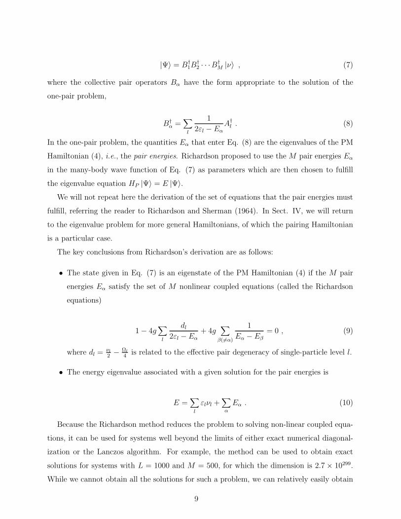
the eigenvalue equation HP |Ψ〉 = E |Ψ〉.We will not repeat here the derivation of the set of equations that the pair energies must
fulfill, referring the reader to Richardson and Sherman (1964). In Sect. IV, we will return
to the eigenvalue problem for more general Hamiltonians, of which the pairing Hamiltonian
is a particular case.
The key conclusions from Richardson’s derivation are as follows:
• The state given in Eq. (7) is an eigenstate of the PM Hamiltonian (4) if the M pair
energies Eα satisfy the set of M nonlinear coupled equations (called the Richardson
equations)
1 − 4g∑
l
dl
2εl − Eα
+ 4g∑
β(6=α)
1
Eα − Eβ
= 0 , (9)
where dl = νl
2− Ωl
4is related to the effective pair degeneracy of single-particle level l.
• The energy eigenvalue associated with a given solution for the pair energies is
E =∑
l
εlνl +∑
α
Eα . (10)
Because the Richardson method reduces the problem to solving non-linear coupled equa-
tions, it can be used for systems well beyond the limits of either exact numerical diagonal-
ization or the Lanczos algorithm. For example, the method can be used to obtain exact
solutions for systems with L = 1000 and M = 500, for which the dimension is 2.7 × 10299.
While we cannot obtain all the solutions for such a problem, we can relatively easily obtain
9

the lowest few for any value of the coupling constant. This means that we can study the
quantum phase transition for pairing using the Richardson algorithm but not any phase
transitions associated with temperature. To do the latter, we would need to develop the
Thermodynamic Bethe ansatz for application to the pairing model, as will be discussed
further in the summary given in Sect. VII.
B. The Gaudin magnet
Inspired by Richardson’s solution of the PM, and building on his previous work on the
Bethe method for solving one-dimensional problems, Gaudin (1976) proposed a family of
fully integrable and exactly-solvable spin models. The Gaudin models are based on the
SU(2) algebra of the spin operators,
[Kα, Kβ
]= 2iεαβγK
γ , (11)
where Kα = σα (α = 1, 2, 3) are the Pauli matrices.
A quantum model with L degrees of freedom is integrable if there exist L independent,
global Hermitian operators that commute with one another. This condition guarantees the
existence of a common basis of eigenstates for the L operators, called the quantum invariants,
and for their eigenvalues, the constants of motion.
Since the SU(2) algebra has one degree of freedom, the most general set of L Hermitian
operators, quadratic in the spin operators and global in L spins, are
Hi =L∑
j(6=i)=1
3∑
α=1
wαij Kα
i Kαj , (12)
where the wαij are 3L (L − 1) real coefficients. To define an integrable model, i.e., to satisfy
the commutation relations [Hi, Hj] = 0, these coefficients must satisfy the system of algebraic
equations
wαijw
γjk + wβ
jiwγik − wα
ikwβjk = 0 . (13)
Gaudin proposed two conditions to solve this system of equations. The first was anti-
symmetry of the w coefficients,
10

wαij = −wα
ji . (14)
The second was to express the w coefficients as an odd function of the difference between
two real parameters,
wαij = fα (ηi − ηj) , (15)
in order to fulfill Eq. (14).
The most general solution of Eq. (13) subject to Eqs. (14) and (15) can be written in
terms of elliptic functions. We further restrict here to the case in which the total spin in
the z direction, Sz = 12
∑i K
zi , is conserved, i.e., the L operators Hi (Gaudin Hamiltonians)
commute with Sz. Conservation of Sz requires that wxij = wy
ij = Xij and wzij = Yij, in terms
of two new matrices X and Y . In such a case, the integrability conditions of Eq. (13) reduce
to
YijXjk + YkiXjk + XkiXij = 0 . (16)
There are three classes of solutions to Eq. (16):
I. The rational model
Xij = Yij =1
ηi − ηj(17)
II. The trigonometric model
Xij =1
sin (ηi − ηj), Yij = cot (ηi − ηj) (18)
III. The hyperbolic model
Xij =1
sinh (ηi − ηj), Yij = coth (ηi − ηj) (19)
We will hold off presenting details on the solution of the three families of Gaudin models
until Sect. II.D, where we discuss the generalization of the Richardson-Gaudin (R-G) models.
At that point we will see that the solutions of the Gaudin models are based on precisely the
same ansatz as used by Richardson in his solution of the pairing model.
11

The most general integrable spin hamiltonian that can be written as a linear combination
of the Gaudin integrals of motion in Eq. (12) is
H = 2∑
i
ζiHi
=∑
i6=j
(ζi − ζj)Xij
[Kx
i Kxj + Ky
i Kyj
]+ YijK
zi K
zj
.
(20)
The above Hamiltonian, which models a spin chain with long-range interactions, has a
total of 2L free parameters. There are L η′s, which define the X ′s, and L ζ ′s. It can
be readily confirmed that the rational family gives rise to an XXX spin model while the
trigonometric and hyperbolic families correspond to an XXZ spin model. To the best of our
knowledge, there have been no physical applications of the Gaudin magnet, though there
are indications that when the 2L free parameters of the model are chosen at random the
Gaudin magnet behaves as a quantum spin glass (Arrachea and Rozenberg, 2001).
The Richardson model has a natural link to superconductivity and the Gaudin model to
quantum magnetism, both very important concepts in contemporary physics. Despite these
facts, neither model received much attention from the nuclear or condensed-matter commu-
nities for many years. On the other hand, the Gaudin models have played an important role
in aspects of quantum integrability. For a recent reference, see Gould et al. (2002).
C. Integrability of the pairing model
Despite the fact that the Richardson and Gaudin models are so similar, it was not until
the work of Cambiaggio, Rivas and Saraceno (1997) (CRS) that a precise connection was
established. We now discuss their work and show how it provides the necessary missing link.
The key point of CRS was to show that the PM is integrable by finding the set of
commuting Hermitian operators in terms of which the PM Hamiltonian could be expressed
as a linear combination. Finding the complete set of common eigenvectors of those quantum
invariant operators is then equivalent to finding the eigenvectors of the PM Hamiltonian.
In their derivation, they began by introducing a pseudo-spin representation of the pair
algebra, advancing a connection between pairing phenomena and spin physics that had been
pointed out long ago by Anderson (1958).
12

The elementary operators of the pair algebra, defined in terms of the generators of the
SU (2) pseudo-spin algebra, are
K0i =
1
2
∑
m
a†lmalm − 1
4Ωl ,
K+l =
1
2
∑
m
a†lma†
lm =(K−
l
)†. (21)
The operator K+l creates a pair of fermions in time-reversed states. The degeneracy Ωl
of level l is related to a pseudo-spin Sl for that level according to Ωl = 2Sl + 1. The three
operators in Eq. (21) close the SU(2) commutation algebra,
[K0
l , K±l′
]= ±δll′K
±l ,
[K+
l , K−l′
]= 2δll′K
0l . (22)
The SU (2) group for a level l has one degree of freedom and its Casimir operator is
(K0
l
)2+
1
2
(K+
l K−l + K−
l K+l
)=
1
4
(Ω2
l − 1)
. (23)
For a problem involving L single-particle levels, there are obviously L degrees of freedom.
Guided by previous work on the two-level PM, CRS considered the following set of oper-
ators:
Rl = K0l + 2g
∑
l′(6=l)
1
εl − εl′
[1
2
(K+
l K−l′ + K−
l K+l′
)
+ K0l K0
l′
]. (24)
They showed that these operators are (1) Hermitian, (2) global, in the sense that they are
independent of the Hilbert space, (3) independent, in the sense that no one can be expressed
as a function of the others, and (4) commute with one another. Furthermore, there are
obviously as many Rl operators as degrees of freedom. The set of L such operators thus
fulfills the conditions required for the quantum invariants of a fully integrable model. Finally,
they showed that the PM Hamiltonian of Eq. (4) can be written as a linear combination of
the Rl according to
HP = 2∑
l
εlRl + C , (25)
13

where C is an uninteresting constant.
We now return to the relationship between the Richardson PM and the Gaudin models.
This can be done by focussing on Gaudin’s rational model and comparing its quantum
invariants to those of CRS [see Eq. (24)] for the pairing model. As can be readily seen,
the two are very similar except that the quantum invariants of Gaudin’s rational model
are missing a one-body term or equivalently a linear term in the spin operators. As shown
by CRS, this term preserves the commutability of the R operators and therefore generalizes
Gaudin’s rational model. In the following subsection, we discuss the solution of the so-called
generalized Richardson-Gaudin models that emerge when this term is added.
D. Generalized Richardson-Gaudin models
The generalization of the Richardson and Gaudin models we now discuss proceeds along
two distinct lines. First, we no longer limit our discussion to Gaudin’s rational model, but
now generalize to all three types (rational, trigonometric and hyberbolic). We will see that
all three can be generalized by the inclusion of a linear term in the quantum invariants.
Second, we generalize our discussion to include boson models as well as fermion models.
We begin by considering the generalization to boson models. For boson systems, the
elementary operators of the pair algebra are
K0i =
1
2
∑
m
a†lmalm +
1
4Ωl ,
K+l =
1
2
∑
m
a†lma†
lm =(K−
l
)†. (26)
Note the similarity with the fermion pair operators of Eq. (21). The only differences are that
(1) there is a relative minus sign between the two terms in the operator K0, and (2) there
is no longer a restriction to Ωl being even. The latter point follows from the fact that for
bosons a single-particle state can be its own time-reversal partner. As an example, consider
scalar bosons confined to a 3D harmonic oscillator potential, as will be discussed further in
Sect. VI.D. The degeneracy associated with a shell having principal quantum number n is
Ωn = (n+1) · (n+2)/2. The lowest two shells (n = 0 and 1) have odd degeneracies, whereas
the next two (n = 2 and 3) have even degeneracies
The set of operators in Eq. (26) satisfy the commutation algebra
14

[K0
l , K±l′
]= ±δll′K
±l ,
[K+
l , K−l′
]= −2δll′K
0l , (27)
appropriate to SU(1,1).
In subsequent considerations, we will often treat fermion and boson systems at the same
time. To facilitate this, we can combine the relevant SU(2) commutation relations for
fermions and SU(1,1) relations for bosons into the compact form
[K0
l , K±l′
]= ±δll′K
±l ,
[K+
l , K−l′
]= ∓2δll′K
0l . (28)
When both types of systems are being treated together, we follow a convention whereby the
upper sign refers to bosons and the lower sign to fermions.
Following earlier discussion, we now consider the most general Hermitian and number-
conserving operator with linear and quadratic terms,
Rl = K0l + 2g
∑
l′(6=l)
[Xll′
2
(K+
l K−l′ + K−
l K+l′
)
∓ Yll′K0l K
0l′
]. (29)
Note that this is a natural generalization of Eq. (24), but now appropriate to both boson
and fermion systems.
We next look for the conditions that the matrices X and Y in Eq. (29) must satisfy
in order that the R operators commute with one other. Surprisingly, the conditions are
precisely those derived by Gaudin and presented in Eq. (16), despite the fact that the
quantum invariants now include a linear term and that they now represent both boson and
fermion systems.
Here too three families of solutions derive, which can be written in compact form as
Xij =γ
sin [γ (ηi − ηj)], Yij = γ cot [γ (ηi − ηj)] , (30)
where γ = 0 corresponds to the rational model, γ = 1 to the trigonometric model and γ = i
to the hyperbolic model. The three limits are completely equivalent to those presented for
the Gaudin magnet in Eqs. (17-19).
15

The next step is to find the exact eigenstates common to all L quantum invariants given
in Eq. (29),
Ri |Ψ〉 = ri |Ψ〉 . (31)
This can be accomplished by using an ansatz similar to the one used by Richardson [see Eq.
(7)] to solve the PM, namely
|Ψ〉 =M∏
α=1
B†α |ν〉 , B†
α =L∑
i=1
ui (Eα) K+i . (32)
The wave function in Eq. (32) is a product of collective pair operators B†α, which are
themselves linear combinations of the raising operators K+i that create pairs of particles in
the various single-particle states. Note that they are analogous to the Richardson collective
pair operators of Eq. (8).
We now present explicitly the solutions to the eigenvalue equations for the three models.
As we will see, it is possible to present the hyperbolic and trigonometric results in a single
set of compact formulae, by using the notation sn for sin or sinh, cs for cos or cosh and
ct for cot or coth. These are not to be confused with elliptic functions. The rational model
solutions are of a somewhat different structure and thus are presented separately. For each
family, we first give the amplitudes ui that define the collective pairs in terms of the free
parameters ηi and the unknown pair energies Eα, then the set of generalized Richardson
equations that define the pair energies Eα, and finally the eigenvalues ri of the quantum
invariants Ri.
I. The rational model
ui (Eα) =1
2ηi − Eα, (33)
1 ± 4g∑
j
dj
2ηj − Eα∓ 4g
∑
β(6=α)
1
Eα − Eβ= 0 , (34)
ri = di
1 ∓ 2g∑
j(6=i)
dj
ηi − ηj
∓ 4g∑
α
1
2ηi − Eα
. (35)
16

II and III. The trigonometric and hyperbolic models
ui (Eα) =1
sn (Eα − 2ηi), (36)
1 ∓ 4g∑
j
djct(Eα − 2ηj) ± 4g∑
β(6=α)
ct(Eβ − Eα) = 0, (37)
ri = di
1 ∓ 2g
∑
j(6=i)
dj ct (ηi − ηj)
−2∑
α
ct (Eα − 2ηi)
]
. (38)
In Eqs. (33-38), the quantity dl is now given by
dl =νl
2± Ωl
4. (39)
Given a set of parameters ηi and a pairing strength g, the pair energies Eα are obtained
by solving a set of M coupled nonlinear equations, either those of Eq. (34) for the rational
model or those of Eq. (37) for the trigonometric or hyperbolic models. In the limit g → 0,
Eqs. (34, 37) can only be satisfied for Eα → 2ηi. In this limit, the corresponding pair
amplitudes ui(Eα) in Eqs. (33, 36) become diagonal and the states of Eq. (32) reduce to a
product of uncorrelated pairs acting on an unpaired state. The ground state, for example,
involves pairs filling the lowest possible states and no unpaired particles. Excitations involve
either promoting pairs from the lowest paired states to higher ones or by breaking pairs and
increasing the seniority. In this way, we can follow the trajectories of the pair energies Eα
that emerge from Eqs. (34, 37) as a function of g for each state of the system.
For boson systems the pair energies are always real, whereas for fermion systems the
pair energies can either be real or can arise in complex conjugate pairs. In the latter case,
there can arise singularities in the solution of Eqs. (34, 37) for some critical value of the
pairing strength gc, when two or more pair energies acquire the same value. It was shown by
Richardson (1965) that each of these critical g values is related to a single-particle level i and
that at the critical point there are 1−2di pair energies degenerate at 2ηi. These singularities
of course cancel in the calculations of energies, which do not show any discontinuity in the
vicinity of the critical points. However, the numerical solution of the nonlinear equations
17

(34) or (37) may break down for values of g close to the singularities, making impractical
the method of following the trajectories of the pair energies Eα from the weak coupling limit
to the desire value of the pairing strength g. Recently, (Rombouts et al., 2003) proposed a
new method based on a change of variables that avoids the singularity problem opening the
possibility of finding numerical solutions in the general case.
The eigenvalues of the R operators, given by Eqs. (35) or (38), are always real since
the pair energies are either real or come in complex conjugate pairs. Each solution of
the nonlinear set of equations produces an eigenstate common to all Ri operators, and
consequently to any Hamiltonian that is written as a linear combination of them. The
corresponding Hamiltonian eigenvalue is the same linear combination of ri eigenvalues.
III. THE ELECTROSTATIC MAPPING OF THE RICHARDSON-GAUDIN MOD-
ELS
We now introduce an exact mapping between the integrable R-G models and a classi-
cal electrostatic problem in two dimensions. Our derivation builds on the earlier work of
Richardson (1977) and Gaudin (1995), who used this electrostatic analogy to show that
the exact solution of the PM Hamiltonian agrees with the BCS approximation in the large-
N limit. For simplicity, we concentrate here on the exact solution for the rational family
(γ = 0). The exact solution of the trigonometric and the hyperbolic families can be reduced
to a set of rational equations by a proper transformation and then also interpreted as a
classical two-dimensional problem (Amico et al., 2002).
Let us assume that we have a two-dimensional (2D) classical system composed of a set
M free point charges and another set of L fixed point charges. For reasons that will become
clear when we use these electrostatic ideas as a means of studying quantum pairing problems,
we will refer to the fixed point charges as orbitons and the free point charges as pairons.
The Coulomb potential due to the presence of a unit charge at the origin is given by the
solution of the Poisson equation
∇2V (r) = −2πδ (r) . (40)
The Coulomb potential V (r) that emerges from this equation depends on the space
dimensionality. For one, two and three dimensions, respectively, the solutions are
18

V (r) ∼
r
ln (r)
1/r
1D
2D
3D
(41)
In 3D, the Coulomb potential has the usual 1/r behavior, but in 2D it is logarithmic. In
practice, there are no 2D electrostatic systems. However, there are cases of long parallel
cylindrical conductors for which the end effects can be neglected so that the problem can be
effectively reduced to a 2D plane. In our case, however, we will simply use the mathematical
structure of the idealized 2D problem to obtain useful new insight into the physics of the
quantum many-body pairing problem.
For the purposes of this discussion, we map the 2D xy-plane into the complex plane by
assigning to each point r a complex number z = x+ iy. Let us now assume that the pairons
have charges qα and positions zα, with α = 1, · · · , M , and that the orbitons have charges
qi and positions zi, with i = 1, · · · , L. Since they are confined to a 2D space, all charges
interact with one another through a logarithmic potential. Let us also assume that there is
an external uniform electric field present, with strength e and pointing along the real axis.
The electrostatic energy of the system is therefore
U = eM∑
α=1
qαRe(zα) + eL∑
j=1
qjRe(zj) −L∑
j=1
M∑
α=1
qαqj ln |zi − zα|
−1
2
∑
α6=β
qαqβ ln |zα − zβ| −1
2
∑
i6=j
qiqj ln |zi − zj | . (42)
If we now look for the equilibrium position of the free pairons in the presence of the fixed
orbitons, we obtain the extremum condition
e +∑
j
qj
zj − zα−
∑
β( 6=α)
qβ
zα − zβ= 0 . (43)
It can be readily seen that the Richardson equations for the rational family (34) coincide
with the equations for the equilibrium position of the pairons (43), if the pairon charges are
qα = 1, the pairon positions are zα = Eα, the orbiton charges qi are equal to the effective
level degeneracies di (which for the ground configuration are ±Ωi/4), the orbitons positions
are zi = 2ηi, and the electric field strength is e = ± 14g
.
19

As a reminder, the ηi’s are free parameters defining the integrals of motion from which
the generalized R-G Hamiltonian is derived [see Eq. (15)]. In the case of the pure PM
Hamiltonian, which is a specific Hamiltonian in the rational family, they are the single-
particle energies of the active levels. In any subsequent discussion in which they are used,
we will thus refer to them as effective single-particle energies.
Table I summarizes the relationship between the quantum PM and the classical elec-
trostatic problem implied by the above analogy. From the above discussion, we see that
solving the Richardson equations for the pair energies Eα is completely equivalent to finding
the stationary solutions for the pairon positions in the analogous classical 2D electrostatic
problem.
TABLE I: Analogy between a quantum pairing problem and the corresponding 2D classical
electrostatic problem.
Quantum Pairing Model Classical 2D Electrostatic Picture
Effective single particle energy ηi Orbiton position zi = 2ηi
Effective orbital degeneracy di Orbiton charge qi = di
Pair energy Eα Pairon position zα = Eα
Pairing strength g Electric field strength e = ± 14g
Assuming that the real axis is vertical and the imaginary axis horizontal, and taking
into account that the orbiton positions are given by the real single-particle energies, it is
clear that they must lie on the vertical axis. The pairon positions are not of necessity
constrained to the vertical axis, but rather must be reflection symmetric around it. This
reflection symmetry property can be readily seen by performing complex conjugation on
the electrostatic energy functional (42). As a consequence, a pairon must either lie on the
vertical axis (real pair energies) or must be part of a mirror pair (complex pair energies).
The various stationary pairon configurations can be readily traced back to the weakly
interacting system (g → 0). In this limit, the pairons for a fermionic system are distributed
around (and very near to) the orbitons, thereby forming compact artificial atoms. The num-
ber of pairons surrounding orbiton i cannot exceed |2di|, as allowed by the Pauli principle,
i.e. we cannot accommodate in a single level more particles than its degeneracy permits. The
lowest-energy (ground-state) configuration corresponds to distributing the pairons around
20

the lowest position orbitons consistent with the Pauli constraint. We then let the system
evolve gradually with increasing g until we reach its physical value. Of course, the Pauli
limitation does not apply to boson systems, which will also be discussed in the applications.
To illustrate how the analogy applies for a specific quantum pairing problem involving
fermions, we consider the atomic nucleus 114Sn. This is a semi-magic nucleus, which can be
modelled as 14 valence neutrons occupying the single-particle orbits of the N = 50−82 shell.
Furthermore, it can be meaningfully treated in terms of a pure PM Hamiltonian with single-
particle energies extracted from experiment. We will return to this problem briefly in Sect.
VI.B. For now we simply want to use this problem to illustrate the relationship between the
quantum parameters and the electrostatic parameters for the analogous classical problem.
In Table II, we list the relevant single-particle orbits of the 50 − 82 shell in the third
column, their corresponding single-particle energies in the first column and the associated
degeneracies in the second. Each level corresponds to an orbiton in the electrostatic problem,
with the position of the orbiton given in the fourth column (at twice the single-particle energy
of the corresponding single-particle level). Note that this is always pure real, meaning that
in the 2D plot each orbiton has y = 0. Finally, in the fifth column we give the charge of the
orbiton, which is simply related to the degeneracy of the level according to the prescription
in Table I.
TABLE II: Relationship between the quantum pairing problem for the nucleus 114Sn and
the corresponding 2D classical problem. The notation “s.p.” is shorthand for
“single-particle”. The s.p. energies are in MeV .
s.p. energy s.p. degeneracy s.p. level/orbiton orbiton position orbiton charge
0.0 6 d5/2 0.0 −1.5
0.22 8 g7/2 0.44 −2.0
1.90 2 s1/2 3.80 −0.5
2.20 4 d3/2 4.40 −1.0
2.80 12 h11/2 5.60 −3.0
To illustrate the weak-pairing limit discussed above, we show in Fig. 1 the pairon positions
associated with the electrostatic solution for 114Sn calculated for a pairing strength of g =
−0.02 MeV , well below the strength at which the superconducting phase transition sets in.
21
Solid lines connect each pairon to its nearest neighbor. As we can readily see, the seven
pairons in this case indeed distribute themselves very near to the lowest two orbitons, with
three forming an artificial atom around the d5/2 and four forming an artificial atom around
the g7/2.
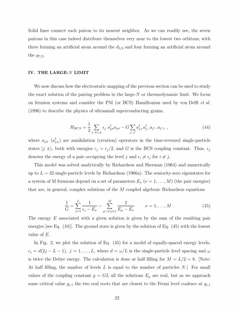
IV. THE LARGE-N LIMIT
We now discuss how the electrostatic mapping of the previous section can be used to study
the exact solution of the pairing problem in the large-N or thermodynamic limit. We focus
on fermion systems and consider the PM (or BCS) Hamiltonian used by von Delft et al.
(1996) to describe the physics of ultrasmall superconducting grains,
HBCS =1
2
∑
j σ=±
ǫj a†jσajσ − G
∑
j j′a†
j+a†j−aj′−aj′+ , (44)
where aj± (a†j±) are annihilation (creation) operators in the time-reversed single-particle
states |j ±〉, both with energies εj = ǫj/2, and G is the BCS coupling constant. Thus, ǫj
denotes the energy of a pair occupying the level j and ǫi 6= ǫj for i 6= j.
This model was solved analytically by Richardson and Sherman (1964) and numerically
up to L = 32 single-particle levels by Richardson (1966a). The seniority-zero eigenstates for
a system of M fermions depend on a set of parameters Eν (ν = 1, . . . , M) (the pair energies)
that are, in general, complex solutions of the M coupled algebraic Richardson equations
1
G=
L∑
j=1
1
ǫj − Eν
−M∑
µ=1(6=ν)
2
Eµ − Eν
ν = 1, . . . , M . (45)
The energy E associated with a given solution is given by the sum of the resulting pair
energies [see Eq. (10)]. The ground state is given by the solution of Eq. (45) with the lowest
value of E.
In Fig. 2, we plot the solution of Eq. (45) for a model of equally-spaced energy levels,
ǫj = d(2j − L − 1), j = 1, . . . , L, where d = ω/L is the single-particle level spacing and ω
is twice the Debye energy. The calculation is done at half filling for M = L/2 = 8. [Note:
At half filling, the number of levels L is equal to the number of particles N .] For small
values of the coupling constant g = GL all the solutions Eµ are real, but as we approach
some critical value gc,1 the two real roots that are closest to the Fermi level coalesce at gc,1
22

and for g > gc,1 develop into a complex conjugate pair. The same phenomenon happens to
other roots as g is further increased, until eventually all of the roots form complex pairs.
This fact was observed by Richardson (1977) and Gaudin (1995) and suggested a way to
analyze systems with a large number of particles, where the exact solution must converge
asymptotically to the BCS solution.
Figure 3 shows the solutions to Eq. (45) for a system with a much larger number of
particles, M = N/2 = 100 pairs, and for three values of g. For g = 1.5, the roots Eµ form
an arc which ends at the points 2λ ± 2i∆, where λ is the BCS chemical potential and ∆
the BCS gap. For g = 1.0 and 0.5, the set of roots consist of two pieces, one formed by an
arc Γ with endpoints 2λ ± 2i∆ which touches the real axis at some point εA, and a set of
real roots along the segment [−ω, εA]. As g decreases, the latter segment gets progressively
larger while the arc becomes smaller and eventually shrinks to a point when g = 0.
The solid lines in the figure are the results obtained from the algebraic equations derived
by Gaudin (1995) in the large-N limit. Note that they are in excellent agreement with the
results obtained by numerically solving Eq. (45).
We now show how to make the connection between the large-N limit of the PM problem
and BCS theory more precise, by applying the electrostatic analogy introduced in Sect. III.
We will consider the limit in which L → ∞, while keeping fixed the following quantities:
G =g
L, ρ =
M
L. (46)
Assuming that the pair energies organize themselves into an arc Γ which is piecewise
differentiable and symmetric under reflection on the real axis, Eq. (45) (the Richardson
equation) in the continuum limit is converted into the integral equation
∫
Ω
ρ(ǫ) dǫ
ǫ − ξ− P
∫
Γ
r(ξ′) |dξ′|ξ′ − ξ
− 1
2G= 0, ξ ∈ Γ, (47)
where ρ(ǫ) is the energy density associated with the energy levels that lie in the interval
Ω = [−ω, ω] and satisfies
∫
Ωρ(ǫ)dǫ =
L
2, (48)
while r(ξ) is the density of the roots Eµ that lie in the arc Γ and satisfies
23

∫
Γr(ξ) |dξ| = M, (49)
∫
Γξ r(ξ)|dξ| = E. (50)
The last equation is a consequence of Eq. (10). The solution of Eq. (47) was given by
Gaudin (1995) using techniques of complex analysis. We now summarize his main results,
which from a different perspective were also given by Richardson (1977). A detailed deriva-
tion of the continuum limit together with a comparison with numerical results for large but
finite systems was presented by Roman et al. (2002).
Introducing an “electric field”, and studying its properties in the vicinity of the arc Γ,
one can show that Eq. (47) yields the well-known BCS gap equation
∫
Ω
ρ(ǫ) dǫ√
( ǫ2− λ)2 + ∆2
=1
G, (51)
that Eq. (49) becomes the equation for the chemical potential
M =∫
Ω
1 −ǫ2− λ
√( ǫ
2− λ)2 + ∆2
ρ(ǫ)dǫ, (52)
and that Eq. (50) gives the BCS expression for the ground-state energy,
E = −∆2
G+
∫
Ω
1 −ǫ2− λ
√( ǫ
2− λ)2 + ∆2
ρ(ǫ) ǫ dǫ. (53)
Thus by using the electrostatic analogy for the quantum pairing problem we are able to
demonstrate how the BCS equations emerge naturally in the large-N limit.
V. THE ELEMENTARY EXCITATIONS OF THE BCS HAMILTONIAN
Most of the studies to date of excited states of the BCS Hamiltonian [see Eq. (44)] based
on Richardson’s exact solution have dealt with a subclass of these states, namely those
obtained by breaking a single Cooper pair. In a case involving doubly-degenerate levels
only, the levels in which the broken pair reside can no longer be occupied by the collective
pairs. Those levels are thus blocked and this is reflected in the Richardson equations by them
having effective degeneracy dl = 0. For more general pairing problems, with degeneracies
24

larger than 2, a broken pair will not completely block a single-particle level, but rather will
increase the seniority νl of the level and give rise to a reduced effective degeneracy di = νi
2−Ωi
4.
There is also another class of collective excitations that arises without changing the seniority.
These excitations, known in nuclear physics as pairing vibrations, correspond to the different
solutions of the Richardson equations for a given seniority configuration νi.
In a mean-field treatment of the same Hamiltonian, the lowest such excitations of both
types correspond to two quasi-particle states in BCS approximation, which are then mixed
by the residual interaction in Random Phase Approximation (RPA). While this bears no
obvious resemblance to the Richardson approach for these elementary excitations, it is clear
that they should coincide in the large-N limit.
To investigate this relation, we focus, for simplicity, on the BCS Hamiltonian of Eq. (44)
and study systematically its excited states for systems with a fixed number of particles. Once
we know the excited states, we can try to interpret them in terms of elementary excitations
characterized by definite quantum numbers, statistics and dispersion relations. A generic
excited state will them be given by a collection of elementary excitations.
The elementary excitations within the exact Richardson approach are associated with the
number of pair energies NG, either real or in complex conjugate pairs, that in the large-g
limit stay finite within the interval between neighboring single-particle levels (Roman et al.,
2003; Yuzbashyan et al., 2003). We display this behavior in Fig. 4 for the ground state
(GS) and the first two excited states for a system with L = 40 single-particle levels at half
filling (M = 20) as a function of g. Note that for the ground state all pair energies become
complex and their real parts go to infinity as the coupling strength becomes infinite. Thus
NG = 0 for this state. Correspondingly we find that for the first and second excited states
the number of pair energies that remain finite are NG = 1 and 2, respectively.
In the large-g limit, the pair energies that stay finite (Efν ) satisfy the Gaudin equation
L∑
j=1
1
ǫj − Efν
−NG∑
µ=1(6=ν)
2
Efµ − Ef
ν
= 0 , ν = 1, . . . , NG, (54)
while the remaining M − NG pair energies (Eiν) go to infinity and are the solution of the
generalized Stieltjes problem encountered by Shastry and Dhar (2001) in the study of the
excitations of the ferromagnetic Heisenberg model,
25
1
g+
L
Eiν
+M−NG∑
µ=1(6=ν)
2
Eiµ − Ei
ν
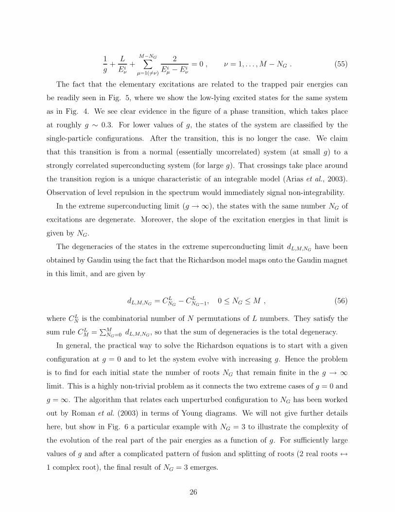
= 0 , ν = 1, . . . , M − NG . (55)
The fact that the elementary excitations are related to the trapped pair energies can
be readily seen in Fig. 5, where we show the low-lying excited states for the same system
as in Fig. 4. We see clear evidence in the figure of a phase transition, which takes place
at roughly g ∼ 0.3. For lower values of g, the states of the system are classified by the
single-particle configurations. After the transition, this is no longer the case. We claim
that this transition is from a normal (essentially uncorrelated) system (at small g) to a
strongly correlated superconducting system (for large g). That crossings take place around
the transition region is a unique characteristic of an integrable model (Arias et al., 2003).
Observation of level repulsion in the spectrum would immediately signal non-integrability.
In the extreme superconducting limit (g → ∞), the states with the same number NG of
excitations are degenerate. Moreover, the slope of the excitation energies in that limit is
given by NG.
The degeneracies of the states in the extreme superconducting limit dL,M,NGhave been
obtained by Gaudin using the fact that the Richardson model maps onto the Gaudin magnet
in this limit, and are given by
dL,M,NG= CL
NG− CL
NG−1, 0 ≤ NG ≤ M , (56)
where CLN is the combinatorial number of N permutations of L numbers. They satisfy the
sum rule CLM =
∑MNG=0 dL,M,NG
, so that the sum of degeneracies is the total degeneracy.
In general, the practical way to solve the Richardson equations is to start with a given
configuration at g = 0 and to let the system evolve with increasing g. Hence the problem
is to find for each initial state the number of roots NG that remain finite in the g → ∞limit. This is a highly non-trivial problem as it connects the two extreme cases of g = 0 and
g = ∞. The algorithm that relates each unperturbed configuration to NG has been worked
out by Roman et al. (2003) in terms of Young diagrams. We will not give further details
here, but show in Fig. 6 a particular example with NG = 3 to illustrate the complexity of
the evolution of the real part of the pair energies as a function of g. For sufficiently large
values of g and after a complicated pattern of fusion and splitting of roots (2 real roots ↔1 complex root), the final result of NG = 3 emerges.
26

These results show the non-trivial nature of the elementary excitations of the pairing
model, as exemplified by their non-trivial counting. As noted above, the elementary excita-
tions satisfy an effective Gaudin equation. They also satisfy a dispersion relation similar to
that of Bogolioubov quasiparticles. For these reasons, this new type of elementary excitation
has been called gaudinos by Roman et al. (2003). An interesting problem, which has been
partially addressed by Yuzbashyan et al. (2003), would be to analyze in detail the relation
between gaudinos and Bogolioubov quasiparticles for large systems.
VI. APPLICATIONS
A. Ultrasmall superconducting grains
Anderson (1959) made the conjecture that superconductivity must disappear for metallic
grains when the mean level spacing d, which is inversely proportional to the volume, is
of the order of the superconducting (SC) gap in bulk, ∆. A simple argument supporting
this conjecture is that the ratio ∆/d measures the number of electronic levels involved in
the formation of Cooper pairs, so that when ∆/d ≤ 1 there are no active levels accessible
to build pair correlations. Apart from some theoretical studies, this conjecture remained
largely unexplored until the recent fabrication of ultrasmall metallic grains.
Ralph, Black and Tinkham (1997) (RBT), in a series of experiments, studied the super-
conducting properties of ultrasmall Aluminium grains at the nanoscale. These grains have
radii ∼ 4-5 nm, mean level spacings d ∼ 0.45 mev, Debye energies ωD ∼ 34 mev and charging
energies EC ∼ 46 mev. Since the bulk gap of Al is ∆ ∼ 0.38 mev, this satisfies Anderson’s
condition, d ≥ ∆, for the possible disappearance of superconductivity. Moreover the large
charging energy EC implies that these grains have a fixed number of electrons, while the
Debye frequency gives an estimate of the number of energy levels involved in pairing, namely
Ω = 2ωD/d ∼ 150, which is rather small. Among other things, RBT found an interesting
parity effect, similar to what is known to occur in atomic nuclei, whereby grains with an
even number of electrons display properties associated with a SC gap, while the odd grains
show gapless behavior.
These experimental findings produced a burst of theoretical activity focused on the study
of the pairing Hamiltonian [Eq. (44)] with equally spaced levels, i.e., εj = jd. Many
27

different approaches were used to study this model including: i) BCS approximation pro-
jected on parity (von Delft et al., 1996), ii) number-conserving BCS approximation (PBCS)
(Braun and von Delft, 1998), iii) Lanzcos diagonalization with up to Ω = 23 energy levels
(Mastellone et al., 1998), iv) Perturbative Renormalization Group combined with small di-
agonalization (Berger and Halperin, 1998), v) the Density Matrix Renormalization Group
(DMRG) with up to Ω = 400 levels (Dukelsky and Sierra, 1999), etc. [For a review on this
topic, see von Delft and Ralph (2001).] Following this flurry of work, it was suddenly real-
ized that the pairing model under investigation had in fact been solved exactly a la Bethe by
Richardson long before. This came as a surprise and led to a posteriori confirmation of the
results obtained by the “exact” numerical methods, namely Lanzcos Diagonalization and
the DMRG. Moreover, the rediscovery of the Richardson solution produced other important
new developments, including generalization of its solution, new insight from the point of
view of integrable vertex models, connection with Conformal Field Theory, Chern-Simons
Theory, etc. [For a review, see Sierra (2001)].
Returning to the application of the Richardson solution to ultrasmall superconducting
grains, we shall focus on two quantities, the condensation energy and the Matveev-Larkin
parameter (Matveev and Larkin, 1997). The condensation energy is the difference between
the ground state energy of the pairing Hamiltonian and the energy of the Fermi state (FS),
namely the Slater determinant obtained by simply filling all levels up to the Fermi surface.
It is given by
ECb = EGS
b − 〈FS|HBCS|FS〉 , (57)
where b = 0 for even-parity grains and b = 1 for those with odd parity. In the BCS solution,
appropriate when the number of electrons N is very large, the leading-order behavior of ECb
is given by −∆2/(2d), where ∆ is the BCS gap in bulk and d scales as 1/N , suggesting
that ECb is independent of the parity b of the system. However, an odd ultrasmall grain
has a single electron occupying the level nearest to the Fermi energy. One can easily show
that this electron decouples from the dynamics of the pairing Hamiltonian, since the pairing
interaction only scatters pairs from energy levels that are doubly occupied to those that are
empty. Hence the single electron only contributes through its free energy. Furthermore,
since there is one less active level at the Fermi energy, it is harder for the pairing interaction
to overcome the gap and the total energy thus increases. This is the physical origin of the
28

parity effect in superconducting grains.
Recall that the BCS gap in bulk is given by ∆ = dN/ sinh(1/g), with g = 0.224 for
Aluminum grains. The BCS result is obtained by solving the gap equation with a finite
number of energy levels N . For even grains, there is a critical value of the ratio dc0/∆ = 3.53,
above which there is no solution to the gap equation. If the grains are odd, the singly
occupied (“blocked”) level must be eliminated from the Hamiltonian, and the critical ratio
becomes dc1/∆ = 0.89. The fact that this is smaller than the even critical ratio indicates that
odd grains are less superconducting than even grains. Thus BCS provides an explanation
of the parity effect observed by RBT. At the same time, it suggests the existence of an
abrupt crossover between the superconducting regime and the normal state, as conjectured
originally by Anderson.
However, the BCS ansatz does not have a definite number of particles, which it only fixes
on average. Though irrelevant for a macroscopic sample, this can be important for systems
with a small number of particles where fluctuations in the phase of the superconducting
order parameter may destroy the superconductivity. For this reason, Braun and von Delft
(1998) considered the PBCS state, which includes number projection and thus does not suffer
from this limitation. There are several important differences between the results obtained
with number projection (PBCS) and without (BCS). Firstly, the condensation energies ECb
from the PBCS ansatz are much lower than those from a corresponding BCS treatment.
Secondly, the sharp transition between the SC regime and the fluctuation-dominated (FD)
regime that arises in BCS is smoothed out by PBCS. Nevertheless, some BCS features
survive the inclusion of number projection, particularly for odd grains. Lastly, in contrast
to BCS, there is always a solution to the PBCS equations.
In the upper panel of Fig. 7, we compare the results of the condensation energy for even
and odd grains as a function of the grain size calculated in the PBCS approximation and
exactly. The exact solution shows a completely smooth SC/FD transition, although one can
still talk about two asymptotic regimes which match near the level spacing for which the
Anderson criterion d/∆ ∼ 1 is satisfied.
Another characterization of the parity effect is in terms of the gap parameter, which
measures the difference between the GS energy of an odd grain and the mean energy of the
neighboring even grains obtained by adding and removing one electron,
29

∆ML = E1(N) − 1
2(E0(N + 1) + E0(N − 1)) . (58)
The lower panel in Fig. 7 compares the value of ∆ML/∆ computed at the level of PBCS
approximation and exactly. Both curves show a minimum in this quantity as a function
of d/∆. This latter feature was first conjectured by Matveev and Larkin (1997) which
is why the associated gap is called the Matveev-Larkin parameter. It was subsequently
confirmed by Mastellone et al. (1998) using the Lanczos method, by Berger and Halperin
(1998) using the Perturbative Renormalization Group combined with small diagonalization,
by Braun and von Delft (1998) using the PBCS method, and by Dukelsky and Sierra (2000)
using the DMRG method. The shape of the exact curve, which is identical to that obtained
using the DMRG, is rather smooth as compared with the PBCS method. This can be
interpreted as a suppression of the even-odd parity effect.
Richardson’s exact solution of the PM can also be used to study the interplay of random-
ness and interactions in a non-trivial model, by examining the effect of level statistics on
the SC/FD crossover, as reflected for example in the location of the critical level spacing.
There was an earlier study of the latter question by Smith and Ambegaokar (1996) using
the BCS approach, who concluded that randomness enhances pairing correlations. More
specifically, they compared the results for a pairing model with a random spacing of levels
(distributed according to a gaussian orthogonal ensemble) with one having uniform spacings.
What they showed is that for both models the BCS theory gives rise to an abrupt SC/FD
crossover, that the random-spacing Hamiltonian produces a lower correlation energy ECb
than the corresponding uniform-spacing model, and that the average value of the critical
level spacing in the model based on random splittings is larger than the corresponding value
for the uniform-spacing model. As noted earlier, however, the mean-field BCS theory pro-
duces an abrupt vanishing of ECb that is not present in more sophisticated treatments. This
raises the question of whether the conclusions they found regarding the role of randomness
may be an artifact of the BCS approach.
Indeed, the exact results shown in Fig. 8 for random levels show that the SC/FD crossover
is as smooth as for the case of uniformly-spaced levels. This means, remarkably, that even
in the presence of randomness, pairing correlations never vanish, no matter how large d/∆
becomes. Quite the contrary, the randomness-induced lowering of EC is found to be strongest
in the FD regime.
30

B. A pictorial representation of pairing in a two-dimensional lattice
We next apply the electrostatic analogy to a model of electrons in a two-dimensional lat-
tice with a residual pairing interaction (Dukelsky et al., 2001). Assuming a nearest-neighbors
hopping term, the single-electron energies in momentum space are εk = −2 (cos kx + cos ky),
with kσ = 2πnσ/P and −P/2 ≤ nσ < P/2. In this expression, σ = x, y and P is the
number of sites on each side of the square lattice. In the numerical example that follows,
we consider a 6 × 6 square lattice at half filling (M = 18) with a constant and attractive
pairing Hamiltonian for which εk = ηk. Table III shows the corresponding information on
the positions and charges of the orbitons in the subspace of seniority-zero states.
Table III: Positions and charges of the orbitons for an attractive 2D pairing model.
2εk −8 −6 −4 −2 0 2 4 6 8
−Ωk/4 −1/2 −2 −2 −2 −5 −2 −2 −2 −1/2
Figure 9 shows the equilibrium positions of the pairons associated with the ground-state
solution for three values of g. The orbitons are represented by open circles with radii
proportional to their charges, and the pairons are represented by solid circles. For each
pairon in the figure, we draw a line connecting it to the one that is closest to it.
In the limit of weak pairing (g = −0.040), 5 pairons are very near the half-filled orbiton
that is located at the Fermi energy (E = 0) and has charge −5. The other 13 pairons are
distributed close to the lowest four orbitons, consistent with the Pauli principle. There is one
near the lowest and four near each of the next three. This part of the figure suggests a picture
whereby for weak pairing the pairons organize themselves as artificial atoms around their
corresponding orbitons. As g increases, the pairons repel, causing the atoms to expand. For
g = −0.064 the two orbitons closest to the Fermi energy have lost their pairons which have
now linked up with the five that are near to the third orbiton. [We can make this linkage more
precise by drawing lines that connect each pairon with its nearest neighbor.] We refer to this
grouping of 13 pairons as a cluster, as it arises from the pairons that originally comprised
three atoms. The remaining 5 pairons are still attached to their orbitons, as artificial atoms.
By g = −0.130, the cluster has grown to the point that all 18 pairons are trapped in it.
We claim that this delocalization effect in the classical problem, from independent atoms to a
collective cluster, is a pictorial reflection of the transition from a normal to a superconducting
31

system in the quantum problem. In the extreme superconducting limit, as reflected in the
figure by the g = −0.130 panel, all pairons are behaving collectively and have lost their
memory of the orbitons from which they arose. In the corresponding quantum problem,
there are a set of Cooper pairs that likewise behave collectively and have lost their connection
to specific single-particle orbits.
Similar results have been reported by Dukelsky et al (2002) for the problem of pairing
between alike nucleons in atomic nuclei. The analysis was for two isotopes of Sn, including
the isotope 114Sn briefly alluded to in Sect. III. There too the superconducting phase tran-
sition was seen to be associated with a transition from isolated atoms to a cluster in the
analogous electrostatic picture. Furthermore, there too the transition to full superconduc-
tivity was seen to develop in steps, depending on the single-particle levels that play a role
in producing the pair correlations and their energy hierarchy.
The analysis of pairing in nuclei reported by Dukelsky et al (2002) assumed a pure PM
interaction. Of course, this is just an approximation to the true nuclear interaction in the
Jπ = 0+ channel. Nevertheless, we expect that the general features of the transition to su-
perconductivity should be the same even for a more realistic pairing interaction. It is in fact
possible to build greater flexibility into the nuclear structure analysis, while still preserving
the electrostatic analogy, by considering more general exactly-solvable Hamiltonians of the
rational family.
C. Electrostatic image of interacting boson models
As an example of the use of the electrostatic mapping for a finite boson system, we now
discuss the phenomenological Interacting Boson Model (IBM) of nuclei (Iachello and Arima,
1980). The IBM captures the collective dynamics of nuclear systems by representing corre-
lated pairs of nucleons with angular momentum L by ideal bosons with the same angular
momentum. In its simplest version, known as IBM1, there is no distinction between protons
and neutrons and only angular momentum L = 0 (s) and L = 2 (d) bosons are retained.
We will use the electrostatic image to study the properties of a second-order quantum
phase transition that arises in the IBM1 from a vibrational system with U(5) symmetry
to a gamma-unstable deformed system with O(6) symmetry. This phase transition can be
modelled by the one-parameter IBM1 Hamiltonian
32
H = nd +x
2P †P , (59)
where nd =∑
µ d†µdµ, P † = s†s† − ∑
µ (−1)µ d†µd
†−µ, s† creates a boson with angular mo-
mentum L = 0, d†µ creates a boson with angular momentum L = 2 and z-projection µ
(−2 ≤ µ ≤ 2), and x is the ratio of the pairing strength g to the single-particle splitting
εd − εs. The parameter x can be varied from x = 0 (the U(5) limit) to x = ∞ (the O(6)
limit). Equation (59) is an example of an exactly-solvable repulsive pairing Hamiltonian,
and the second-order nature of the phase transition it describes has been recently attributed
to quantum integrability (Arias et al., 2003).
The electrostatic problem that corresponds to this quantum boson model consists of two
orbitons with positive charges qs = 1/4 and qd = 5/4 (see Sect. III). Both the s and d
orbitons are located on the real axis, with the s located at position 0.0 and the d at position
2.0. There are M pairons with positive unit charge that interact with the orbitons and
with one another and that feel an external electric field pointing downwards with strength
1/x. In the ground-state configuration, the pairons are constrained to move between the
two orbitons.
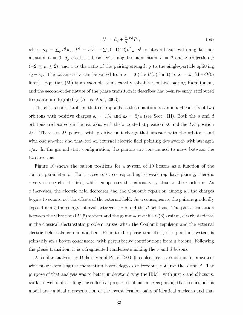
Figure 10 shows the pairon positions for a system of 10 bosons as a function of the
control parameter x. For x close to 0, corresponding to weak repulsive pairing, there is
a very strong electric field, which compresses the pairons very close to the s orbiton. As
x increases, the electric field decreases and the Coulomb repulsion among all the charges
begins to counteract the effects of the external field. As a consequence, the pairons gradually
expand along the energy interval between the s and the d orbitons. The phase transition
between the vibrational U(5) system and the gamma-unstable O(6) system, clearly depicted
in the classical electrostatic problem, arises when the Coulomb repulsion and the external
electric field balance one another. Prior to the phase transition, the quantum system is
primarily an s boson condensate, with perturbative contributions from d bosons. Following
the phase transition, it is a fragmented condensate mixing the s and d bosons.
A similar analysis by Dukelsky and Pittel (2001)has also been carried out for a system
with many even angular momentum boson degrees of freedom, not just the s and d. The
purpose of that analysis was to better understand why the IBM1, with just s and d bosons,
works so well in describing the collective properties of nuclei. Recognizing that bosons in this
model are an ideal representation of the lowest fermion pairs of identical nucleons and that
33
there are not just 0+ and 2+ pairs, a natural question to ask is: Why can we ignore the higher
angular momentum pairs/bosons when dealing with nuclear collective properties? Part of
the answer is contained in the dominant quadrupole-quadrupole neutron-proton interaction,
which is known to favor the lowest 0+ and 2+ pair degrees of freedom. Dukelsky and Pittel
(2001) suggested another mechanism, based on an analysis of a generalized boson model con-
taining all even angular momenta up to some maximum and interacting via a repulsive boson
pairing interaction. The latter is a means of simulating the repulsive interaction between
bosons that arises due to the Pauli principle between the fermion (nucleon) constituents of
which they are comprised. Using the Richardson solution of this model, they showed that
a repulsive boson pairing interaction can only correlate two boson degrees of freedom, and
that these should be the lowest two, the s and the d. More recently, this result has been
interpreted by means of the electrostatic mapping (Pittel and Dukelsky, 2003). Even in the
presence of many boson degrees of freedom and thus many orbitons, the collective pairons
are always confined to lie between the lowest two, i.e., between the s and the d.
D. Application to a boson system confined by a harmonic oscillator trap
We now consider the problem of a set of bosons confined to a harmonic oscillator trap and
subject to a boson pairing interaction. We claim that such a Hamiltonian cannot realistically
describe the physics of a confined boson system, for the following reason. Looking back at
the commutators of the pair operators A†l given in Eq. (2), we see that they are normalized to
the square root of the degeneracy Ωl of the level l. Thus, the PM Hamiltonian of Eq. (4) has
a pairing matrix element proportional to√
ΩlΩl′ . In a three-dimensional harmonic confining
potential, these degeneracies are in turn proportional to l2, where l plays the role of the
principal quantum number and the summation in the pair operators of Eq. (1) now include
both the orbital and the magnetic quantum numbers. On the other hand, the single-boson
energies εl for such a confining potential are linear in l. Thus, a boson pairing interaction in
the presence of an oscillator confining trap would have the net effect of scattering boson pairs
to high-lying levels with greater probability than to low-lying levels, producing unphysical
occupation numbers.
To numerically test this conjecture, we have solved the Richardson equations [Eq. (34)]
for a system of 1000 bosons (M = 500) trapped in a three-dimensional harmonic oscillator
34

(Ωl = (l + 1) (l + 2) /2 and εl = hω(l + 3/2))with a cutoff at 101/2hω (L = 50 single boson
levels). Following Richardson (1968), the occupation numbers can be calculated as
〈nl〉 =
⟨∂HP
∂εl
⟩
=∑
p
∂Ep
∂εl(60)
From Eqs. (4) and (34), a set of M coupled nonlinear equations in terms of M new
unknowns are obtained, which when solved give the L occupation numbers. For details of
the derivation , see Richardson (1968).
In Fig. 11, we show the occupation numbers versus the single-boson energies in units of
hω for a pairing strength of g = −0.0025. We have excluded the occupation of the l = 0
condensed boson state from the figure, since it lies outside the scale of the figure. The overall
depletion is 0.21, which gives an occupation of the l = 0 state of n0 = 790 bosons. The figure
clearly shows that the depletion is unphysically dominated by the high-lying (i.e., high-l)
levels, due to the nature of the pair coupling matrix elements discussed above.
We can use the freedom we have in choosing the parameters ηl entering in the definition
of the R operators to obtain a more physical exactly-solvable model. In order to cancel the
unphysical dependence of the pair coupling matrix elements on the degeneracies, we choose
the η’s so that ηl = (εl)3. Then, the new Hamiltonian, which is given by the associated
linear combination of R′s, will be
H = 2∑
l
εlRl = C +∑
l
εlnl +∑
l 6=l′Vll′
[A†
l Al′ − nlnl′
], (61)
where
C =1
2
∑
l
εlΩl −1
4
∑
l 6=l′Vll′ΩlΩl′ ,
εl = εl −∑
l′(6=l)
Vll′Ωl′ ,
Vll′ =g
2
1
ε2l + ε2
l′ + εlεl′. (62)
Taking into account that εl is proportional to l, the two-body matrix elements in Eq. (62)
cancel the dependence on the degeneracies in the effective pair coupling matrix elements.
Thus the above Hamiltonian should be more appropriate when modelling a harmonically-
confined boson system with a pairing-like interaction.
35

The interaction in Eq. (62) has the nice feature that its two-body matrix elements
decrease with the number of shells, as one would expect in general. It has the particular
property that the interactions of the pair- and density-fluctuations are strictly the same
but opposite in sign. The energy eigenvalues of this Hamiltonian can be obtained from the
eigenvalues rl of the associated Rl operators as E = 2∑
l εl rl, with the end result being
E =1
2
∑
l
εlΩl −1
4
∑
l 6=l′Vll′ΩlΩl′ − 2g
∑
lp
εlΩl
2ε3l − Ep
. (63)
Note that the first two terms in the energy eigenvalues of Eq. (63) exactly cancel the constant
term C in Eq. (61).
We have solved the Richardson equations for the Hamiltonian of Eq. (62), i.e., with
ηl = (εl)3, for the same system considered above, namely M =500 and L =50. In Fig. 12,
we show the occupation numbers for g = −1.0, for which the overall depletion factor is 0.245.
They display a reasonable physical pattern, with the occupancies decreasing monotonically
with increasing single-boson energy. A comparison between the exact results and such
approximations as Hartree-Fock-Bogolyubov theory or its number-conserving variants will
be the subject of future work.
When the same modified form for the Hamiltonian, but with repulsive pairing, was con-
sidered, a highly unexpected feature was found (Dukelsky and Schuck, 2001). Figure 13
shows the occupation numbers of the first and second levels versus the scaled pairing in-
teraction x = 2Mg/hω for the same system as above (M = 500, L = 50). At the critical
value of the scaled interaction, xc = 1, the normal ground-state boson condensate suddenly
changes into a new phase in which the bosons occupy the l = 0 and the l = 1 levels, with
the occupation of all other levels negligible.
This new phase is characterized in the large-N limit by having two macroscopically oc-
cupied states, thus representing a fragmented condensate. It is commonly accepted since
the work of Nozieres and Saint James (1982) that for confined systems fragmentation can-
not occur in systems of scalar bosons with repulsive interactions. This might be the first
example of fragmentation in a confined boson system.
36

VII. SUMMARY AND OUTLOOK
In this Colloquium, we have reviewed recent efforts to develop exactly-solvable models of
the Richardson-Gaudin type and have discussed how these models have been used to provide
valuable insight into the physics of systems with strong pair correlations. We began with a
brief review of Richardson’s original treatment of the pairing model and Gaudin’s related
treatment of the Gaudin magnet and then showed how they could be generalized to several
classes of exactly-solvable models that still preserve a pairing-like structure.
A very attractive feature of these models is that one can establish an exact analogy
between the associated quantum many-body problem and the classical physics of a two-
dimensional electrostatic system. This feature, which was originally appreciated by both
Richardson and Gaudin, has now been generalized to all such exactly-solvable models.
The solution to a classical problem is typically amenable to simple geometrical interpre-
tation, which can then be used to give an alternative perspective on the quantum model
from which it derives. This has been used in several examples we have discussed, both for
boson and fermion systems. It provides a new perspective on how superconductivity arises
in fermion models and also an interesting new perspective on a second-order quantum phase
transition that arises in the nuclear Interacting Boson Model.
Another important outcome of the classical electrostatic analogy is that it facilitates
a treatment of these models in the thermodynamic limit. Not surprisingly, it shows that
BCS theory is indeed the correct large-N limit of the fermion pairing model with attractive
interactions.
The generalization of Richardson and Gaudin’s models was first discussed in the context
of the physics of small metallic grains, as a means of obtaining exact solutions to the BCS
Hamiltonian appropriate to such systems in cases where numerical diagonalization was out
of the question. As discussed in some detail in this Colloquium, the existence of a method
of exact solution for this model provides important insight into the detailed physics present
when the size of the system gets small enough so that superconductivity disappears. Neither
BCS theory nor number-projected BCS theory can capture the physics of the phase transition
acceptably.
The new families of exactly-solvable models that we have discussed are based on the
algebras SU(2) (for fermion systems) or SU(1,1) (for boson systems). These two algebras
37

have a pseudo-spin representation in terms of fermion pairs or boson pairs, respectively. All
applications to date and all that we have therefore discussed are based on these represen-
tations of the associated algebras. At the same time, the SU(2) group has other possible
representations in terms of spins operators or two-level atoms which have not yet been
exploited.
Perhaps, the most important feature of the exactly-solvable R-G models is the enormous
freedom within an integrable family. For a given set of L single-particle levels (or orbits),
we can define an exactly-solvable Hamiltonian in terms of L + 1 ηi and g parameters that
enter in the definition of the associated quantum invariants [Eqs. (29,30)], and an additional
set of L parameters εi that define a Hamiltonian as a linear combination of the quantum
invariants. The models therefore contain 2L + 1 free parameters, which allows enormous
flexibility in constructing a general pairing-like interaction tailored to the physical problem
of interest (Dukelsky et al., 2003). In contrast, most other exactly-solvable models have
either no free parameters (the Heisenberg model), one free parameter (the XXZ model, the
Hubbard model, or the Elliott model), or just a few free parameters (the three dynamical
symmetry limits of the nuclear Interacting Boson Model). We reported here one particu-
larly interesting use of this flexibility, namely to model the physics of bosons confined to a
harmonic trap. A pure pairing interaction has the anomalous feature that it scatters pairs
of bosons preferentially to high-energy states. By exploiting the flexibility of the general-
ized R-G models, it was possible to find a more physically-meaningful Hamiltonian for such
systems, which nevertheless was still exactly solvable. Analysis of this new model led to a
suggestion that confined boson systems can exist in a fragmented state, contrary to prior
expectations.
All the application reported discussed in this Colloquium made use of generalized R-G
models of the so-called rational class. Other interesting applications within this class of
models should certainly be sought.
A potentially interesting example concerns the properties of the pairing phase transition in
finite Fermi systems at finite temperature. There has already been important work reported
on this topic (see, for example, Dean and Hjorth-Jensen (2003) and reference therein). As
noted earlier, the exact solution of the pairing model can be derived from the Algebraic
Bethe ansatz. It is natural, therefore, to study the Thermodynamic Bethe ansatz, which
provides the exact finite temperature description of short-range 1D integrable models, to
38

see whether it could be extended for application to integrable pairing models. If so, this
would allow for an exact treatment of the finite temperature properties of such systems as
nuclei, ultrasmall superconducting grains and degenerate Fermi gases.
Another important topic that has recently received attention (Dean and Hjorth-Jensen,
2003) is the study of the low-energy properties of quantum many-body systems with random
interactions and in particular with random pairing interactions. Though random pairing
interactions in general have chaotic properties, there is an important subset of integrable
pairing hamiltonians that have a large number of free parameters which can be chosen
randomly. Some of the physical consequences of randomly chosen pairing interactions in
the general chaotic regime and within the integrable subset of pairing models have been
reported recently by Volya et al. (2002) and Relano et al. (2004), respectively.
We also expect interesting applications to ensue for the trigonometric and hyperbolic
models. As one example, the trigonometric model was used by Gaudin (1976) to derive the
limit of an exactly-solvable model of the interaction of a two-level atomic system with an
external oscillator field. This kind of model could lead to a generalization of the celebrated
Jaynes-Cummings model. Using techniques similar to the Algebraic Bethe ansatz derivation
of the Richardson model, exactly-solvable models for boson atomic-molecule systems and
two coupled Bose-Einstein condensates have recently been found ( Links et al., 2003). Based
on these arguments, we believe that R-G models could have a promising future in Quantum
Optics and in the study of dilute Fermi and Bose gases.
Another area of great interest is the generalization of R-G models based on the SU(2) or
SU(1,1) algebras to larger algebras. Some work has already been reported along these lines
(Asorey et al , 2002). A complete solution for models with O(5) or SU(4) symmetries could
lead to interesting applications for nuclear systems with N ≈ Z, where it is important to
explicitly include the isospin degree of freedom. It could also provide useful insight into the
properties of high Tc superconductors (Wu et al., 2003; Zhang , 1997). Though in previous
works Richardson (1966b, 1967) proposed an exact solution for pairing Hamiltonians with
these two group symmetries, recent work by Pan and Draayer (2002) indicates that his
solution is invalid for systems with more than two pairs. Moreover, Links et al. (2002) and
Guan et al. (2002) have found different solutions for the same problems. More work is clearly
required along these lines.
In closing, the use of exactly-solvable Richardson-Gaudin models has already provided
39

significant new and important insight into the properties of many diverse quantum systems,
ranging from atomic nuclei to electronic systems in condensed matter. We are optimistic
that many more exciting applications are still to come.
Acknowledgments
This work was supported in part by the Spanish DGI under grants # BFM2000-1320-
C02-01/02 and in part by the US National Science Foundation under Grant Nos. PHY-
9970749 and PHY-0140036. We wish to express our gratitude to Carlos Esebbag, Jose
Marıa Roman and Peter Schuck, all of whom contributed significantly to the work reported
in this Colloquium.
References
Amico, L., A. Di Lorenzo, and A. Osterloh, 2001, Phys. Rev. Lett. 86, 5759.
Amico, L., G. Falci, and R. Fazio, 2001, J. Phys. A 34, 6425.
Amico, L., A. Di Lorenzo, A. Mastellone, A. Osterloh, and R. Raimondi, 2002, Ann. Phys. (N.Y.)
299, 228.
Anderson, P. W., 1958, Phys. Rev. 112, 1900.
Anderson, P. W., 1959, J. Phys. Chem. Solids 11, 28.
Arias, J. E., J. Dukelsky, and J. E Garcıa–Ramos, 2003, Phys. Rev. Lett. 91, 162502.
Arrachea, L., and M. J. Rozenberg, 2001, Phys. Rev. Lett. 86, 5172, and private communication.
Asorey, M., F. Falceto, and G. Sierra, 2002, Nucl. Phys. B 622, 593.
Baldo, M., J. Cugnon, A. Lejeune, and U. Lombardo, 1990, Nucl. Phys. A 515, 409.
Bang, J., and J. Krumlimde, 1970, Nucl. Phys. A 141, 18.
Bardeen, J., L. N. Cooper, and J. R. Schrieffer, 1957, Phys. Rev. 108, 1175.
Berger, S. D., and B. I Halperin, 1998, Phys. Rev. B 58, 5213.
Bethe, H. A., 1931, Z. Phys. 71, 265.
Braun, F., and J. von Delft, 1998, Phys. Rev. Lett. 81, 4712.
Calogero, F., 1962, J. Math. Phys. 10, 2191.
Cambiaggio, M. C., A. M. F. Rivas, and M. Saraceno, 1997, Nucl. Phys. A 624, 157.
Dean, D. J., and M. Hjorth-Jensen, 2003, Rev. Mod. Phys. 75, 607.
40

Dietrich, K., H. J Mang, and J. H Pradal, 1964, Phys. Rev. B 135, 22.
Dukelsky, J., and G. Sierra, 1999, Phys. Rev. Lett. 83, 172.
Dukelsky, J., and G. Sierra, 2000, Phys. Rev. B 61, 12302.
Dukelsky, J., C. Esebbag, and P. Schuck, 2001, Phys. Rev. Lett. 87, 66403.
Dukelsky, J., and P. Schuck, 2001, Phys. Rev. Lett. 86, 4207.
Dukelsky, J., and S. Pittel, 2001, Phys. Rev. Lett. 86, 4791.
Dukelsky, J., C. Esebbag, and S. Pittel, 2002, Phys. Rev. Lett. 88, 062501.
Dukelsky, J., J. M Roman, and G. Sierra, 2003, Phys. Rev. Lett. 90, 249803.
Elliott, J. P., 1958, Proc. Roc. Soc. A242, 128, 562.
Gaudin, M., 1976, J. Phys. (Paris) 37, 1087.
Gaudin, M., 1995, Etats propres et valeurs propres de l’Hamiltonien d’appariement (Les Editions
de Physique).
Gould, M. D., Y.-Z. Zhang, and S.-Y. Zhao, 2002, Nucl. Phys. B 630, 492.
Greiner, M., C. A. Regal, and D. S Jin, 2003, Naure (London) 426, 537.
Guan, X.-W., A. Foerster, J. Links, and H.-Q. Zhou 2002, Nucl. Phys. B 642, 501.
Ha, Z. N. C., 1996, Quantum Many-Body Systems in One Dimension, (World Scientific).
Haldane, F. D. M., 1981, J. Phys. C 14, 2585.
Haldane, F. D. M., 1988, Phys. Rev. Lett. 60, 635.
Hasegawa, M., and S. Tasaki, 1987, Phys. Rev. C 35, 1508.
Hasegawa, M., and S. Tasaki, 1993, Phys. Rev. C 47, 188.
Heiselberg, H., 2003, Phys. Rev. A 68, 053616.
Heritier, M., 2001, Nature (London) 414, 31.
Iachello, F., and A. Arima, 1980, The Interacting Boson Model (Cambridge University Press).
Jochim, S., et al., Science 302, 5653.
Links, J., H.-Q. Zhou, M. D. Gould, and R. H. McKenzie 2002, J. Phys. A 35, 6459.
Links, J., H.-Q. Zhou, R. H. McKenzie, and M. D. Gould, 2003, J. Phys. A 36, R63.
Luttinger, J. M., 1963, J. Math. Phys. 15, 609.
Mastellone, A., G. Falci, and R. Fazio, 1998, Phys. Rev. Lett. 80, 4542.
Matveev, K. A., and A. I. Larkin, 1997, Phys. Rev. Lett. 78, 3749.
Nozieres, P., and D. Saint James, 1982, J. Phys. (Paris) 43, 1133.
Pan, F., and J. P. Draayer, 2002, Phys. Rev. C 66, 044314.
41

Pittel, S., and J. Dukelsky, 2003, eprint nucl-th/0309020.
Ralph, D. C., C. T. Black, and M. Tinkham, 1997, Phys. Rev. Lett. 78, 4087.
Regal, C. A., M. Greiner, and D. S. Jin, 2004, Phys. Rev. Lett. 92, 040403.
Relano, A., J. M. G. Gomez, J. Retamosa, and J. Dukelsky, 2004, eprint nlin.CD/0402011.
Richardson, R. W., 1963a, Phys. Lett. 3, 277.
Richardson, R. W., 1963b, Phys. Lett. 5, 82.
Richardson, R. W., and N. Sherman, 1964, Nucl. Phys. B 52, 221.
Richardson, R. W., 1965, J. Math. Phys. 6, 1034.
Richardson, R. W., 1966a, Phys. Rev. 141, 949.
Richardson, R. W., 1966b, Phys. Rev. 144, 874.
Richardson, R. W., 1967, Phys. Rev. 159, 792.
Richardson, R. W., 1968, J. Math. Phys. 9, 1327.
Richardson, R. W., 1977, J. Math. Phys. 18, 1802.
Roman, J. M, G. Sierra, and J. Dukelsky, 2002, Nucl. Phys. B 634, 483.
Roman, J. M, G. Sierra, and J. Dukelsky, 2003, Phys. Rev. B 67, 064510.
Rombouts, S., D. Van Neck, and J. Dukelsky, 2003, eprint nuc-th/0312070.
Schechter, M., Y. Imry, Y. Levinson, and J. von Delft, 2001, Phys. Rev. B 63, 214518.
Shastry, B. S., 1988, Phys. Rev. Lett. 60, 639.
Shastry, B. S., and A. Dhar, 2001, J. Phys. A 34, 6197.
Sierra, G., 2000, Nucl. Phys. B 572, 517.
Sierra, G., J. Dukelsky, G. G. Dussel, J. von Delft,and F. Braun, 2000, Phys. Rev. B 61, 11890.
Sierra, G., 2001, eprint hep-th/0111114.
Sigrist, M., and K. Ueda, 1991, Rev. Mod. Phys. 63, 239.
Smith, R. A., and V. Ambegaokar, 1996, Phys. Rev. Lett. 77, 4962.
Sutherland, B., 1971, J. Math. Phys. 12, 246.
Tomonaga, S., 1950, Prog. Theor. Phys. 5, 544.
Volya, A., V. Zelevinsky, and B. A. Brown, 2002, Phys. Rev. C 65, 054312.
von Delft, J., D. S. Golubev, W. Tichy, and A. D. Zaikin, 1996, Phys. Rev. Lett. 77, 3189.
von Delft, J., and D. C. Ralph, 2001, Phys. Rep. 345, 61.
von Delft, J., and R. Poghossian, 2002, Phys. Rev. B 66, 134502.
Wu, L.-A., M. W. Guidry, Y. Sun, and C.-L. Wu, 2002, Phys. Rev. B 67, 014515.
42

Yuzbashyan, E. A., A. A. Baytin, and B. L. Altshuler, 2003, eprint cond-mat/0305635.
Zhang, S.-C., 1997, Science 275, 1089.
Zhou, H.-Q., J. Links, R. H. McKenzie, and M. D. Gould, 2002, Phys. Rev. B 65, 060502.
Figures
-0.6 -0.4 -0.2 0.0 0.2 0.4 0.6
-0.2
0.0
0.2
0.4
0.6
Im(E)
g=-0.02 MeV
Re(
E)
FIG. 1 Two-dimensional representation of the pairon positions in 114Sn for a pure PM Hamiltonian
with single-particle energies as given in Table II and with g = −0.02 MeV .
0 0.2 0.4 0.6 0.8 1 1.2
-12
-8
-4
0
4
8
12
ImE
µ
0 0.2 0.4 0.6 0.8 1 1.2g
0
2
4
6
8
10
12
14
16
ReE
µ
43

FIG. 2 Evolution of the real and imaginary parts of Eµ(g), in units of the mean level spacing
d = ω/L, for the equally-spaced model with M = L/2 = 8, as a function of the coupling constant
g. For convenience, the energy levels are chosen in this figure as ǫj = 2j. The dashed curves in
the lower half are an average of the two neighboring real energies. Following the critical point, this
turns into the real part of the energy of the resulting complex conjugate pair. From Roman et al.
(2002).
FIG. 3 Plot of the roots Eµ for the equally-spaced pairing model in the complex ξ-plane. The
discrete symbols denote the numerical values for M = 100. All energies are in units of ω. From
Roman et al. (2002).
0 0.5 1-44
-40
-36
-32
-28
-24
-20
-16
-12
-8
-4
0
4
Re
Eµ /
d
Ground State (a)
0 0.5 1g
1 excitation (b)
0 0.5 1 1.5
2 excitations (c)
FIG. 4 Real part of Eµ in units of the mean level spacing d for the equally-spaced pairing model
with M = L/2 = 20 pairs and NG = 0, 1, 2 excitations. From Roman et al. (2003).
44

0 0.5 1 1.5g
0
4
8
12
16
20
24
28
32
36
40
44
48
52
56
60
64
68
Eex
c / d
1 excitation2 excitations3 excitations
FIG. 5 Lowest 44 excitation energies Eexc = E − EGS in units of the mean level spacing d for
M = 20 pairs at half filling. From Roman et al. (2003).
F
F
0 0.5 1 1.5g
-44
-40
-36
-32
-28
-24
-20
-16
-12
-8
-4
0
4R
e E
µ / d
(2)
(1)
(b)(a)
FIG. 6 An illustration of the algorithm for determining the number of roots NG, for a case with
NG = 3. a) Top: Initial state at g = 0, where each solid circle (•) denotes a level occupied by a
pair, each empty cicle () denotes an empty level, and the vertical dashed line with an F near it
denotes the position of the Fermi surface. Bottom: The associated Young diagram. b) Real part
of Eµ. From Roman et al. (2003).
45

-5.0
-4.5
-4.0
-3.5
-3.0
-2.5
-2.0
-1.5
b=0 Exact
b=1 PBCS
b=1 Exact
b=0 PBCS
EC b/ ~ ∆
0.0 0.5 1.0 1.5 2.0 2.5 3.0 3.5 4.0
0.3
0.4
0.5
0.6
0.7
0.8
0.9
1.0
∆ ML/ ~ ∆
d/ ~∆
Exact
PBCS
FIG. 7 Calculated results for ultrasmall superconducting grains as a function of the grain size.
The upper panel gives the condensation energies ECb for even (b = 0) and odd (b = 1) grains
calculated using PBCS and exact wave functions. The lower panel gives the Matveev-Larkin gap,
∆ML, obtained in PBCS calculations (Braun and von Delft, 1998) and in exact calculations. The
quantity ∆ that scales the condensation energy, the Matveev-Larkin gap and the mean level spacing
d is the BCS gap in bulk.
46

0 1 2 3 4Level spacing d/
-5
-4
-3
-2
Con
dens
atio
n en
ergy
[
]∆∼
∆∼
uniformly spacedrandomly spaced
s=1/2
s=0
FIG. 8 Exact even and odd condensation energies ECb for uniform equally-spaced levels (dashed
line), and the ensemble average energies 〈ECb 〉 for random-spaced levels (solid line). The height of
the fluctuation bars gives the variances δECb . The results are plotted as a function of the mean
level spacing, d, scaled by the BCS gap in bulk, ∆. From Sierra et al. (2000).
-8-6-4-202
g=-0.064
Re(
e)
-8-6-4-202
g=-0.040Re(
e)
-8 -6 -4 -2 0 2 4 6 8
-8-6-4-202
Im(e)
g=-0.130Re(
e)
FIG. 9 Two-dimensional representation of the positions of the orbitons and pairons corresponding
to a 6× 6 lattice at half filling, for three selected values of g. The orbitons are represented by open
circles and the pairons by solid circles, with radii proportional to their charges.
47

0.0 0.2 0.4 0.6 0.8 1.0
0.0
0.5
1.0
1.5
2.0
s
d
Pai
ron
posi
tion
x
FIG. 10 Evolution of the pairon positions as a function of the scaled strength parameter x for
a model with 10 s and d bosons subject to a Hamiltonian with linear single-boson energies and
a repulsive boson pairing interaction. The circles at x = 0 denote the positions of the s and d
orbitons.
0 5 10 15 20 25 30 35 40 45 501.5
2.0
2.5
3.0
3.5
4.0
4.5
5.0
5.5
Occ
upat
ion
Num
bers
l
FIG. 11 Occupation numbers for 1000 bosons confined in 50 harmonic oscillator shells and inter-
acting via a pure pairing interaction with strength g = −.0025. The occupation of the l=0 state is
off scale and thus not shown.
0 1 2 3 4 5 6 7 8 9 100
100
200
300
400
500
600
700
800
Occ
upat
ion
Num
bers
l
48

FIG. 12 Occupation numbers for 1000 bosons confined in 50 harmonic oscillator shells and inter-
acting via a renormalized pairing interaction [see Eq. (62)] with g = −1.0.
0.0 0.5 1.0 1.5 2.0 2.5 3.0 3.5 4.00
100200300400500600700800900
1000
n1
n0
Occ
upat
ion
num
bers
x
FIG. 13 Occupation numbers n0 and n1 for 1000 bosons confined to 50 harmonic oscillator shells
and interacting via a repulsive renormalized pairing interaction as a function of the scaled strength
parameter x.
49