Meetup: Cómo monitorizar y optimizar procesos de Spark usando la Spark Web - 28 de Marzo 2017

Proyecto realizado por la alumna:
María del Pilar Romón Peris
Fdo.: …………………… Fecha: ……/ ……/ ……
Autorizada la entrega del proyecto cuya información no es de carácter confidencial
EL DIRECTOR DEL PROYECTO
Henning Skriver
Fdo.: …………………… Fecha: ……/ ……/ ……
Vº Bº del Coordinador de Proyectos
Álvaro Sánchez Miralles
Fdo.: …………………… Fecha: ……/ ……/ ……
RESUMEN
I
UNIVERSIDAD PONTIFICIA COMILLAS
ESCUELA TÉCNICA SUPERIOR DE INGENIERÍA (ICAI)
INGENIERO INDUSTRIAL
RESUMEN
Debido al crecimiento de la población mundial, el sector agrícola se ha convertido
en un factor social y económico muy importante. Este factor hace que el uso de la
tierra y la conservación de recursos naturales sea uno de los grandes retos de la
humanidad. Por esta razón, y para estimar las producciones agrícolas, es necesario
desarrollar métodos para monotorizar el estado de los campos de cultivo y su
estado de desarrollo.
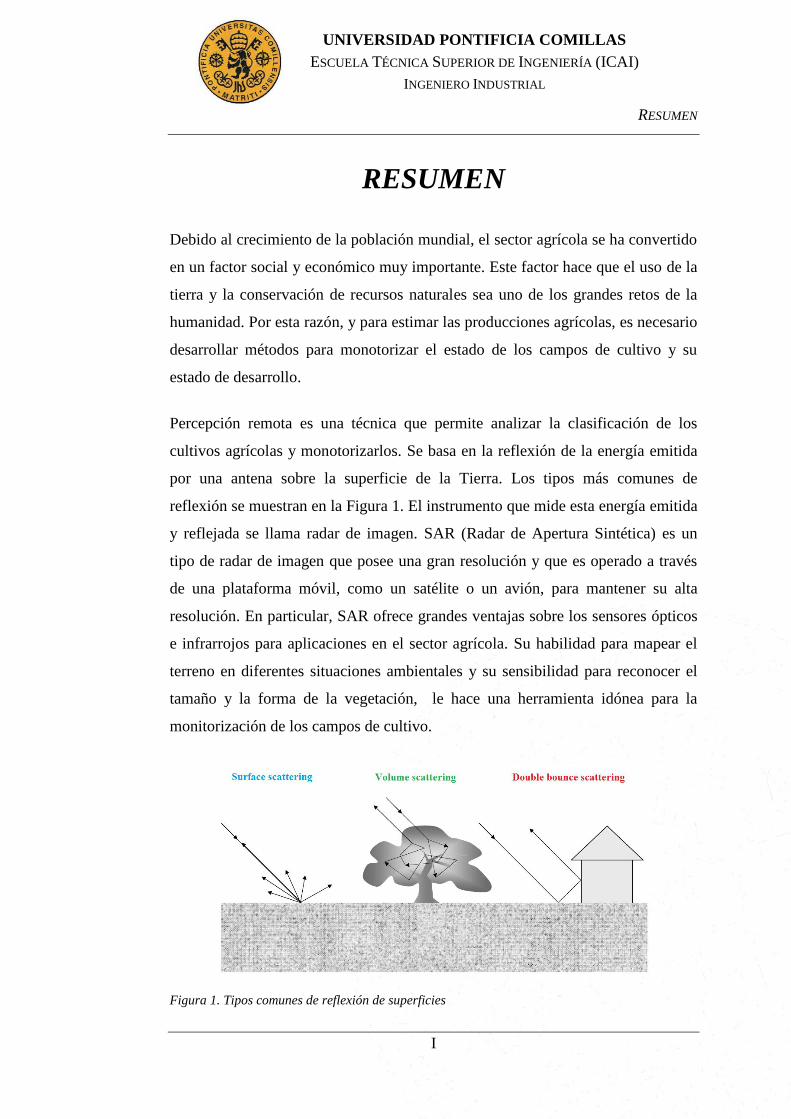
Percepción remota es una técnica que permite analizar la clasificación de los
cultivos agrícolas y monotorizarlos. Se basa en la reflexión de la energía emitida
por una antena sobre la superficie de la Tierra. Los tipos más comunes de
reflexión se muestran en la Figura 1. El instrumento que mide esta energía emitida
y reflejada se llama radar de imagen. SAR (Radar de Apertura Sintética) es un
tipo de radar de imagen que posee una gran resolución y que es operado a través
de una plataforma móvil, como un satélite o un avión, para mantener su alta
resolución. En particular, SAR ofrece grandes ventajas sobre los sensores ópticos
e infrarrojos para aplicaciones en el sector agrícola. Su habilidad para mapear el
terreno en diferentes situaciones ambientales y su sensibilidad para reconocer el
tamaño y la forma de la vegetación, le hace una herramienta idónea para la
monitorización de los campos de cultivo.
Figura 1. Tipos comunes de reflexión de superficies
RESUMEN
II
UNIVERSIDAD PONTIFICIA COMILLAS
ESCUELA TÉCNICA SUPERIOR DE INGENIERÍA (ICAI)
INGENIERO INDUSTRIAL
El objetivo principal de este proyecto es desarrollar e implementar dos métodos
estadísticos basados en la interpretación de imágenes SAR polarimétricas, con la
finalidad de monitorizar y mapear los cultivos agrícolas mostrados en la Figura 2.
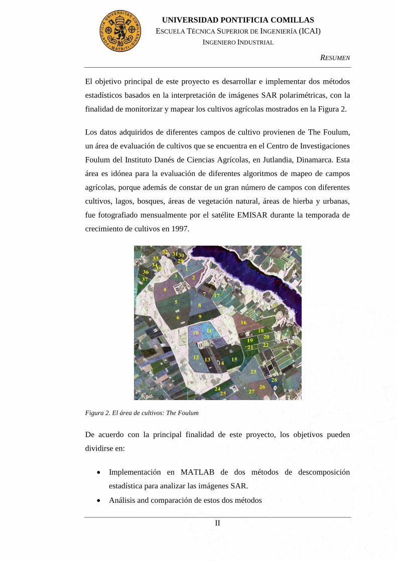
Los datos adquiridos de diferentes campos de cultivo provienen de The Foulum,
un área de evaluación de cultivos que se encuentra en el Centro de Investigaciones
Foulum del Instituto Danés de Ciencias Agrícolas, en Jutlandia, Dinamarca. Esta
área es idónea para la evaluación de diferentes algoritmos de mapeo de campos
agrícolas, porque además de constar de un gran número de campos con diferentes
cultivos, lagos, bosques, áreas de vegetación natural, áreas de hierba y urbanas,
fue fotografiado mensualmente por el satélite EMISAR durante la temporada de
crecimiento de cultivos en 1997.
Figura 2. El área de cultivos: The Foulum
De acuerdo con la principal finalidad de este proyecto, los objetivos pueden
dividirse en:
Implementación en MATLAB de dos métodos de descomposición
estadística para analizar las imágenes SAR.
Análisis and comparación de estos dos métodos
RESUMEN
III
UNIVERSIDAD PONTIFICIA COMILLAS
ESCUELA TÉCNICA SUPERIOR DE INGENIERÍA (ICAI)
INGENIERO INDUSTRIAL
Clasificación de los cultivos de las imágenes SAR del área agrícola
Análisis y evaluación del desarrollo de estos cultivos
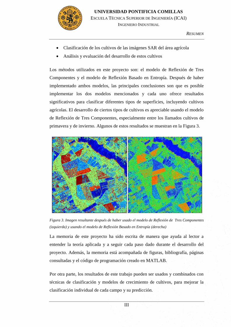
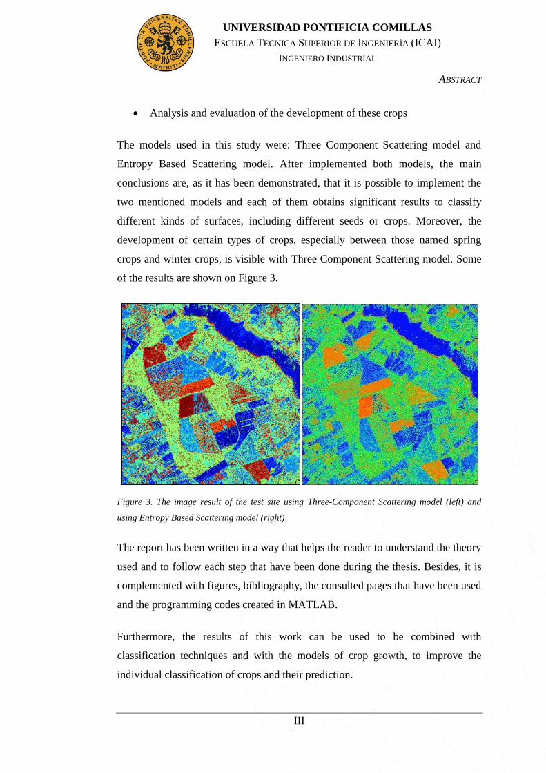
Los métodos utilizados en este proyecto son: el modelo de Reflexión de Tres
Componentes y el modelo de Reflexión Basado en Entropía. Después de haber
implementado ambos modelos, las principales conclusiones son que es posible
implementar los dos modelos mencionados y cada uno ofrece resultados
significativos para clasificar diferentes tipos de superficies, incluyendo cultivos
agrícolas. El desarrollo de ciertos tipos de cultivos es apreciable usando el modelo
de Reflexión de Tres Componentes, especialmente entre los llamados cultivos de
primavera y de invierno. Algunos de estos resultados se muestran en la Figura 3.
Figura 3. Imagen resultante después de haber usado el modelo de Reflexión de Tres Componentes
(izquierda) y usando el modelo de Reflexión Basado en Entropía (derecha)
La memoria de este proyecto ha sido escrita de manera que ayuda al lector a
entender la teoría aplicada y a seguir cada paso dado durante el desarrollo del
proyecto. Además, la memoria está acompañada de figuras, bibliografía, páginas
consultadas y el código de programación creado en MATLAB.
Por otra parte, los resultados de este trabajo pueden ser usados y combinados con
técnicas de clasificación y modelos de crecimiento de cultivos, para mejorar la
clasificación individual de cada campo y su predicción.

ABSTRACT
I
UNIVERSIDAD PONTIFICIA COMILLAS
ESCUELA TÉCNICA SUPERIOR DE INGENIERÍA (ICAI)
INGENIERO INDUSTRIAL
ABSTRACT
Due to global population growth, the agricultural sector is a social and economic
factor very essential. This social and economic factor reflects that land use and the
conservation of natural resources are one of the biggest challenges of humanity.
Therefore, in order to estimate agricultural productions, it is necessary to develop
methods to monitor the status of crops and its stage of development.
Remote sensing is a technique that can analyze the classification of agricultural
crops and monitor the crops. It depends upon measuring the reflection or
scattering of incident energy from earth surface features emitted by an antenna.
Figure 1 shows the three most common scattering mechanisms. The instrument,
that measures this energy emitted by an antenna and reflected by a distant surface,
is an imaging radar. SAR (Synthetic Aperture Radar) is a form of imaging radars
that has a high resolution and it is operated from a moving platform, such a
satellite or aircraft, to achieve its high resolution. In particular, SAR offers great
advantages over the optical and infrared sensors for agricultural applications. Its
ability to map the terrain in different weather situations and it is sensitive to the
size, shape and form of vegetation, makes SAR an adequate tool to monitor
agricultural crops.
Figure 1. Common scattering mechanisms
ABSTRACT
II
UNIVERSIDAD PONTIFICIA COMILLAS
ESCUELA TÉCNICA SUPERIOR DE INGENIERÍA (ICAI)
INGENIERO INDUSTRIAL
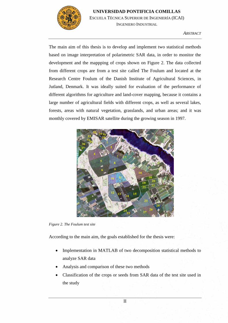
The main aim of this thesis is to develop and implement two statistical methods
based on image interpretation of polarimetric SAR data, in order to monitor the
development and the mappping of crops shown on Figure 2. The data collected
from different crops are from a test site called The Foulum and located at the
Research Centre Foulum of the Danish Institute of Agricultural Sciences, in
Jutland, Denmark. It was ideally suited for evaluation of the performance of
different algorithms for agriculture and land-cover mapping, because it contains a
large number of agricultural fields with different crops, as well as several lakes,
forests, areas with natural vegetation, grasslands, and urban areas; and it was
monthly covered by EMISAR satellite during the growing season in 1997.
Figure 2. The Foulum test site
According to the main aim, the goals established for the thesis were:
Implementation in MATLAB of two decomposition statistical methods to
analyze SAR data
Analysis and comparison of these two methods
Classification of the crops or seeds from SAR data of the test site used in
the study
ABSTRACT
III
UNIVERSIDAD PONTIFICIA COMILLAS
ESCUELA TÉCNICA SUPERIOR DE INGENIERÍA (ICAI)
INGENIERO INDUSTRIAL
Analysis and evaluation of the development of these crops
The models used in this study were: Three Component Scattering model and
Entropy Based Scattering model. After implemented both models, the main
conclusions are, as it has been demonstrated, that it is possible to implement the
two mentioned models and each of them obtains significant results to classify
different kinds of surfaces, including different seeds or crops. Moreover, the
development of certain types of crops, especially between those named spring
crops and winter crops, is visible with Three Component Scattering model. Some
of the results are shown on Figure 3.
Figure 3. The image result of the test site using Three-Component Scattering model (left) and
using Entropy Based Scattering model (right)
The report has been written in a way that helps the reader to understand the theory
used and to follow each step that have been done during the thesis. Besides, it is
complemented with figures, bibliography, the consulted pages that have been used
and the programming codes created in MATLAB.
Furthermore, the results of this work can be used to be combined with
classification techniques and with the models of crop growth, to improve the
individual classification of crops and their prediction.

CONTENTS OF THE REPORT
I
UNIVERSIDAD PONTIFICIA COMILLAS
ESCUELA TÉCNICA SUPERIOR DE INGENIERÍA (ICAI)
INGENIERO INDUSTRIAL
Contents of the report
Part I Report .............................................................................................. 1
Chapter 1 Introduction .................................................................................... 2
1.1 Theory............................................................................................................... 2
1.1.1 Synthetic Aperture Radar (SAR) .................................................................................... 2
1.1.2 Common Scattering Mechanisms ................................................................................... 3
1.1.3 SAR Data ....................................................................................................................... 4
1.1.4 Three Component Scattering Model .............................................................................. 5
1.1.5 Entropy Based Scattering Model.................................................................................... 7
1.1.6 Speckle in SAR images ................................................................................................ 10
1.1.6.1 Speckle filter ........................................................................................................ 11
1.2 Motivation ...................................................................................................... 13
1.3 Objectives ....................................................................................................... 14
1.4 Methodology ................................................................................................... 15
1.5 Sources used and Supporting tools .............................................................. 16
1.5.1 Test site ........................................................................................................................ 16
1.5.2 Data .............................................................................................................................. 18
1.5.3 Programming language: MATLAB ............................................................................. 19
Chapter 2 Implementation ............................................................................. 20
2.1 Speckle filter .................................................................................................. 20
2.2 Three Component Scattering Model ........................................................... 22
2.3 Entropy Based Scattering Model ................................................................. 28
Chapter 3 Results ........................................................................................... 30
3.1 Speckle Filter ................................................................................................. 30
3.2 Three Component Scattering Model ........................................................... 32
3.3 Entropy Based Scattering Model ................................................................. 36

CONTENTS OF THE REPORT
II
UNIVERSIDAD PONTIFICIA COMILLAS
ESCUELA TÉCNICA SUPERIOR DE INGENIERÍA (ICAI)
INGENIERO INDUSTRIAL
3.3.1 Entropy-alpha planes .................................................................................................... 36
3.3.2 Classification of crops .................................................................................................. 38
3.4 Comparison of models ................................................................................... 41
3.4.1 L-band .......................................................................................................................... 41
3.4.2 C-band .......................................................................................................................... 44
3.5 Development of Crops ................................................................................... 46
3.5.1 Beets ............................................................................................................................. 47
3.5.2 Cereals .......................................................................................................................... 50
3.5.2.1 Spring barley ........................................................................................................ 51
3.5.2.2 Winter Wheat ....................................................................................................... 53
3.5.2.3 Rye ....................................................................................................................... 55
3.5.3 Peas .............................................................................................................................. 57
Chapter 4 Conclusions ................................................................................... 60
4.1 Implementation .............................................................................................. 60
4.2 Results............................................................................................................. 61
Chapter 5 Future Work ................................................................................. 62
Bibliography 63
Part II User guide ..................................................................................... 65
Chapter 1 MATLAB Programming .............................................................. 66
Part III Programming code ....................................................................... 69
Chapter 1 Three Component Scattering Model ............................................ 70
Chapter 2 Entropy Based Scattering Model ................................................. 91
Chapter 3 Speckle Filter .............................................................................. 109
Part IV Data results ................................................................................. 120
Chapter 1 Three Component Scattering Model .......................................... 121
1.1 Tables of Powers .......................................................................................... 121
1.1.1 Beets ........................................................................................................................... 121
1.1.2 Grass .......................................................................................................................... 122
1.1.3 Peas ............................................................................................................................ 123

CONTENTS OF THE REPORT
III
UNIVERSIDAD PONTIFICIA COMILLAS
ESCUELA TÉCNICA SUPERIOR DE INGENIERÍA (ICAI)
INGENIERO INDUSTRIAL
1.1.4 Rye ............................................................................................................................. 126
1.1.5 Spring Barley ............................................................................................................. 128
1.1.6 Spring Oats ................................................................................................................. 132
1.1.7 Winter Wheat ............................................................................................................. 133
1.2 Image Result ................................................................................................ 136
1.2.1 April ........................................................................................................................... 136
1.2.2 May ............................................................................................................................ 137
1.2.3 June ............................................................................................................................ 138
1.2.4 July ............................................................................................................................. 139
Chapter 2 Entropy Based Scattering Model ............................................... 140
2.1 Tables of Entropy & Alpha ........................................................................ 140
2.1.1 Beets ........................................................................................................................... 140
2.1.2 Grass .......................................................................................................................... 141
2.1.3 Peas ............................................................................................................................ 142
2.1.4 Rye ............................................................................................................................. 145
2.1.5 Spring Barley ............................................................................................................. 147
2.1.6 Spring Oats ................................................................................................................. 151
2.1.7 Winter Wheat ............................................................................................................. 152
2.2 Entropy Alpha Planes ................................................................................. 155
2.2.1 April ........................................................................................................................... 155
2.2.2 May ............................................................................................................................ 156
2.2.3 June ............................................................................................................................ 157
2.2.4 July ............................................................................................................................. 158
2.3 Image Results ............................................................................................... 159
2.3.1 April ........................................................................................................................... 159
2.3.2 May ............................................................................................................................ 160
2.3.3 June ............................................................................................................................ 161
2.3.4 July ............................................................................................................................. 162

LIST OF FIGURES
IV
UNIVERSIDAD PONTIFICIA COMILLAS
ESCUELA TÉCNICA SUPERIOR DE INGENIERÍA (ICAI)
INGENIERO INDUSTRIAL
List of figures
Figure 1. Common scattering mechanisms ............................................................. 4
Figure 2. Entropy-alpha plane ................................................................................. 9
Figure 3. SAR image with speckle at the left and the same image filtered reducing
the speckle [7] ....................................................................................................... 11
Figure 4. Eight edge-aligned windows. Depending on the edge direction, one of
the eight windows is to be selected ....................................................................... 12
Figure 5. Methodology of the project .................................................................... 15
Figure 6. The Foulum test site ............................................................................... 17
Figure 7. Equivalent number of looks for 8 20x20 homogeneous areas ............... 20
Figure 8. The areas of where var(x) in the SAR image was negative colored in
white ...................................................................................................................... 21
Figure 9. On the right half plane of the plots, the number of pixels for which
surface scatter is assumed to be dominant. All other pixels are assumed to have
double-bounce scatter as a dominant ..................................................................... 22
Figure 10. The histograms represent the amount of pixels corresponding to the
values of in deg when surface is dominant (up) and when
double bounce is dominant (down) ....................................................................... 23
Figure 11. 50 largest values of according to their allocations . 24
Figure 12. 100 largest values of as they are located on the
image ..................................................................................................................... 25
Figure 13. 50 largest values of powers for pixels that correspond to volume and
surface scattering mechanism according to their allocations on the image .......... 26
Figure 14. Histograms of powers of April data at L-band .................................... 27
Figure 15. Entropy-alpha planes in April at C-band ............................................. 28

LIST OF FIGURES
V
UNIVERSIDAD PONTIFICIA COMILLAS
ESCUELA TÉCNICA SUPERIOR DE INGENIERÍA (ICAI)
INGENIERO INDUSTRIAL
Figure 16. Image result in April at C-band, using Entropy Based Scattering model
with uncommon pixels in color white ................................................................... 29
Figure 17. Comparison of HH and VV phase differences from the original data
(up) and filtered data (down). The phase differences were coded by the gray scale
shown above these two images ............................................................................. 31
Figure 18. Powers according to each relevant type of crop in April at C-band (up)
and at L-band (down) ........................................................................................... 32
Figure 19. Image of the test site based on Three Component Scattering model in
April at C-band (up) and at L-band (down) .......................................................... 33
Figure 20. Image result using Three Component Scattering model in May at L-
band. Using only 3 clusters (up) and using 15 clusters (down) ............................ 35
Figure 21. Entropy-alpha planes in May at C-band (up) and at L-band (down) ... 37
Figure 22. Entropy and Alpha according to type of crop in May at C-band (up)
and L-band (down) ................................................................................................ 39
Figure 23. Image based on Entropy Based Scattering model in May, at C-band
(up) and at L-band (down) ..................................................................................... 40
Figure 24. (a) The image result using Three Component Scattering model. (b) The
image result using Entropy Based Scattering model. (c) Areal image with
numbered fields ..................................................................................................... 42
Figure 25. (a) The image result using Three Component Scattering model
(Filtering). (b) The image result using Entropy Based Scattering model (Filtering).
(c) Areal real image with numbered fields ............................................................ 43
Figure 26. C-Band images of the data not filtered and acquired in April with
Three Component Scattering Model (left) and with Entropy Based Scattering
model (right) .......................................................................................................... 45
Figure 27. C-Band image results of filtered data and acquired in April with Three
Component Scattering model (left) with Entropy Based Scattering model (right) 45
Figure 28. Growth stages of beet plants [12] ........................................................ 47

LIST OF FIGURES
VI
UNIVERSIDAD PONTIFICIA COMILLAS
ESCUELA TÉCNICA SUPERIOR DE INGENIERÍA (ICAI)
INGENIERO INDUSTRIAL
Figure 29. Double bounce power of beet crops at C-band: left and, at L-band:
right ....................................................................................................................... 49
Figure 30. Volume power of beet crops at C-band: left, and at L-band: right ...... 49
Figure 31. Surface power of beet crops at C-band: left, and at L-band: right ....... 49
Figure 32. Growth stages of cereal plants [12] ..................................................... 50
Figure 33. Double bounce power of spring barley crops at C-band: left and, at L-
band: right .............................................................................................................. 52
Figure 34. Volume power of spring barley crops at C-band: left and at L-band:
right ....................................................................................................................... 52
Figure 35. Surface power of spring barley crops at C-band: left, and at L-band:
right ....................................................................................................................... 52
Figure 36. Double bounce power of winter wheat crops at C-band: left, and at L-
band: right .............................................................................................................. 54
Figure 37. Volume power of winter wheat crops at C-band: left, and at L-band:
right ....................................................................................................................... 54
Figure 38. Surface power of winter wheat crops at C-band: left, and at L-band:
right ....................................................................................................................... 54
Figure 39. Double bounce power of rye crops at C-band: left, and at L-band: right
............................................................................................................................... 56
Figure 40. Volume power of rye crops at C-band: left and at L-band: right ........ 56
Figure 41. Surface power of rye crops at C-band: left, and at L-band: right ....... 56
Figure 42. Growth stages of pea plants [12] ......................................................... 57
Figure 43. Double bounce power of pea crops at C-band: left, and at L-band: right
............................................................................................................................... 59
Figure 44. Volume power of pea crops at C-band: left, and at L-band: right ....... 59
Figure 45. Surface power of pea crops at C-band: left and at L-band: right ......... 59
Figure 46. C-band of the April acquisition applying Three Component Scattering
model ................................................................................................................... 136

LIST OF FIGURES
VII
UNIVERSIDAD PONTIFICIA COMILLAS
ESCUELA TÉCNICA SUPERIOR DE INGENIERÍA (ICAI)
INGENIERO INDUSTRIAL
Figure 47. L-band of the April acquisition applying Three Component Scattering
model ................................................................................................................... 136
Figure 48. C-band of the May acquisition applying Three Component Scattering
model ................................................................................................................... 137
Figure 49. L-band of the May acquisition applying Three Component Scattering
model ................................................................................................................... 137
Figure 50. C-band of the June acquisition applying Three Component Scattering
model ................................................................................................................... 138
Figure 51. L-band of the June acquisition applying Three Component Scattering
model ................................................................................................................... 138
Figure 52. C-band of the July acquisition applying Three Component Scattering
model ................................................................................................................... 139
Figure 53. L-band of the July acquisition applying Three Component Scattering
model ................................................................................................................... 139
Figure 54. Entropy-alpha planes of the April acquisition at C-band ................... 155
Figure 55. Entropy-alpha planes of the April acquisition at L-band ................... 155
Figure 56. Entropy-alpha planes of the May acquisition at C-band .................... 156
Figure 57. Entropy-alpha planes of the May acquisition at L-band .................... 156
Figure 58. Entropy-alpha planes of the June acquisition at C-band .................... 157
Figure 59. Entropy-alpha planes of the June acquisition at L-band .................... 157
Figure 60. Entropy-alpha planes of the July acquisition at C-band .................... 158
Figure 61. Entropy-alpha planes of the July acquisition at L-band ..................... 158
Figure 62. C-band of the April acquisition applying Entropy Based Scattering
model ................................................................................................................... 159
Figure 63. L-band of the April acquisition applying Entropy Based Scattering
model ................................................................................................................... 159
Figure 64. C-band of the May acquisition applying Entropy Based Scattering
model ................................................................................................................... 160

LIST OF FIGURES
VIII
UNIVERSIDAD PONTIFICIA COMILLAS
ESCUELA TÉCNICA SUPERIOR DE INGENIERÍA (ICAI)
INGENIERO INDUSTRIAL
Figure 65. L-band of the May acquisition applying Entropy Based Scattering
model ................................................................................................................... 160
Figure 66. C-band of the June acquisition applying Entropy Based Scattering
model ................................................................................................................... 161
Figure 67. L-band of the June acquisition applying Entropy Based Scattering
model ................................................................................................................... 161
Figure 68. C-band of the July acquisition applying Entropy Based Scattering
model ................................................................................................................... 162
Figure 69. L-band of the July acquisition applying Entropy Based Scattering
model ................................................................................................................... 162

LIST OF TABLES
IX
UNIVERSIDAD PONTIFICIA COMILLAS
ESCUELA TÉCNICA SUPERIOR DE INGENIERÍA (ICAI)
INGENIERO INDUSTRIAL
List of tables
Table 1: Types of crop and their field number according to Figure 5 ................... 17
Table 2: BBCH scale ............................................................................................. 46
Table 3: Height and BBCH of beet field from April to July ................................. 48
Table 4. Height and BBCH of spring barley field from April to July ................... 51
Table 5: Height and BBCH of winter wheat fields from April to July ................. 53
Table 6: Height and BBCH of rye fields from April to July ................................. 55
Table 7: Height and BBCH of pea fields from April to July ................................ 58

LIST OF SYMBOLS
X
UNIVERSIDAD PONTIFICIA COMILLAS
ESCUELA TÉCNICA SUPERIOR DE INGENIERÍA (ICAI)
INGENIERO INDUSTRIAL
List of symbols
α Complex parameter (Freeman-Durden decomposition)
Average angle (Cloude-Pottier decomposition)
Complex parameter (Freeman-Durden decomposition)
Complex parameter (Freeman-Durden decomposition)
Eigenvalue
Measure of speckle level
Complex parameter (Freeman-Durden decomposition)
b Weighting function
Polarimetric covariance matrix
C1 Function of the first curve of Entropy-alpha plane
C2 Function of the second curve of Entropy-alpha plane
Eigenvector
E {·} Mean operator
Eh Electric field component for polarization h
Ei Incident electric field
Es Scattered electric field
Equivalent number of looks
Ev Electric field component for polarization v
Surface scatter contributions
Double-bounce scatter contributions
Volume scatter contributions
H Entropy (Cloude-Pottier decomposition)
m Multi-look image

LIST OF SYMBOLS
XI
UNIVERSIDAD PONTIFICIA COMILLAS
ESCUELA TÉCNICA SUPERIOR DE INGENIERÍA (ICAI)
INGENIERO INDUSTRIAL
Linear Matrix Transform
N Number of looks
Probability associated to eigenvalue . Called also power
Pd, Pdb Power associated to double bounce scattering
Ps Power associated to surface scattering
Pv Power associated to volume scattering
Scattered Matrix
Shh Complex scattering amplitudes for receive polarization h and transmit
polarization h
Shv Complex scattering amplitudes for receive polarization h and transmit
polarization v
Svh Complex scattering amplitudes for receive polarization v and transmit
polarization h
Svv Complex scattering amplitudes for receive polarization v and transmit
polarization v
Polarimetric coherency matrix
V {·} Variance operator
Variance of the reflectance without speckle noise
Local variance
x Noise-free pixel value
Filtered pixel value
y Center pixel value
Local mean
Z Hermitian matrix
Filtered covariance matrix

LIST OF ACRONYMS
XII
UNIVERSIDAD PONTIFICIA COMILLAS
ESCUELA TÉCNICA SUPERIOR DE INGENIERÍA (ICAI)
INGENIERO INDUSTRIAL
List of acronyms
BBCH Bundesanstalt, Bundessortenamt and CHemical industry
EMISAR Polarimetric Danish airborne SAR system
ENL Equivalent Number of Looks
HH Horizontal Transmit, Horizontal Receive
HV Horizontal Transmit, Vertical Receive
VH Vertical Transmit, Horizontal Receive
SAR Synthetic Aperture Radar
VV Vertical Transmit, Vertical Receive

GLOSSARY
XIII
UNIVERSIDAD PONTIFICIA COMILLAS
ESCUELA TÉCNICA SUPERIOR DE INGENIERÍA (ICAI)
INGENIERO INDUSTRIAL
Glossary
Backscattering: In a scattering problem, backscattering direction refers to the
opposite direction of the incident wave. A backscattering configuration refers to
those situations in which the transmitting and receiving systems are collocated. Booting: It occurs when vegetative plant parts appear in the seed.
Boxcar filter: Spatial filtering consisting of the average of a certain quantity over
a given number of pixels.
Classification: Signal processing technique aiming to cluster the image pixels
which present common characteristics.
Cluster: Group of pixels with the same feature or scattering mechanism.
Coherent decomposition: Any decomposition of the scattering matrix into
simpler scattering mechanisms.
Complex scattering amplitude: Without considering the propagation effects, the
complex scattering amplitude refers to the quotient between the scattered and the
incident fields.
Complex scattering coefficient: The same as complex scattering amplitude.
Correlation coefficient: Magnitude of the complex correlation coefficient of a
pair of complex SAR images.
C-band: Name given to a certain portion of the electromagnetic spectrum,
between 4 to 8 GHz.
Double bounce scattering: It occurs when the wave is reflected in a horizontal
and then in a vertical direction.

GLOSSARY
XIV
UNIVERSIDAD PONTIFICIA COMILLAS
ESCUELA TÉCNICA SUPERIOR DE INGENIERÍA (ICAI)
INGENIERO INDUSTRIAL
Eigen decomposition: It also receives the name of “matrix diagonalization”. For
a square matrix, it consists of the transformation giving as a result a diagonal
matrix. The elements of the resulting diagonal matrix are called eigenvalues,
whereas the columns of the matrix performing the transformation are called
eigenvectors.
Equivalent number of looks (ENL): A quantity employed to describe the
statistics of the speckle noise. The higher its value, the lower the variance of
speckle noise.
Flowering: The process from first flowers open to fruit set is visible.
Germination: The beginning of growth of a seed or crop. The germination of
most crops occurs in response to warmth and water.
Heading: Inflorescence emergence. The process before flowering.
Jones vector: Complex bidimensional vector employed to describe the
polarization of an electromagnetic wave. It contains all the polarization
information except the polarization handedness as it does not contain propagation
information.
L-band: Name given to a certain portion of the electromagnetic spectrum,
between 1 to 2 GHz.
Orthogonality: In elementary geometry, the same as perpendicular. In the case of
a space vector, two elements v and w are said orthogonal if their inner product
equals zero.
Ripening: Maturity of fruit and seed.
Senescence: Deterioration of a seed.
Segmentation: Signal processing technique aiming to divide the image pixels
which present common characteristics.

GLOSSARY
XV
UNIVERSIDAD PONTIFICIA COMILLAS
ESCUELA TÉCNICA SUPERIOR DE INGENIERÍA (ICAI)
INGENIERO INDUSTRIAL
Span: Power received by a fully polarimetric systems. It consists of the addition
of the intensity of the four elements of the scattering matrix.
Speckle: Statistical variation associated with SAR imagery and caused by the
coherent nature of the imaging process.
Stokes vector: Four dimensional real vector able to represent the polarization
state of an electromagnetic wave.
Supervised classification: Classification based on the external help of the user.
This classification scheme is not automatic.
Surface scattering: Scattering mechanism produced by a surface (smooth or
rough).
Synthetic Aperture Radar (SAR): It is a type of radar whose main characteristic
is the use of relative motion between an antenna and its target region to provide
consistent long-term distinctive signal and to obtain a good spatial resolution of
the target.
Tillering: It refers to the production of tillers. This process occurs when multiple
stems (tillers) are produced starting from the initial single tiller.
Unsupervised classification: Classification without any external help of the user.
This classification scheme is considered fully automatic.
Volume scattering: Scattering mechanism produced in a cloud of particles, it is
generally due to trees or vegetation.

REPORT
1
UNIVERSIDAD PONTIFICIA COMILLAS
ESCUELA TÉCNICA SUPERIOR DE INGENIERÍA (ICAI)
INGENIERO INDUSTRIAL
Part I REPORT

REPORT - Introduction
2
UNIVERSIDAD PONTIFICIA COMILLAS
ESCUELA TÉCNICA SUPERIOR DE INGENIERÍA (ICAI)
INGENIERO INDUSTRIAL
Chapter 1 INTRODUCTION
Remote sensing depends upon measuring the reflection or scattering of incident
energy from earth surface features. If the incident energy is in the optical range of
wavelengths – i.e. in the visible or near infrared – it is scattered largely by the
surface of the material being imaged. Sometimes there is penetration into a
medium, such as short wavelengths into water.
Because the wavelength of the microwave energy used in radar remote sensing is
so long by comparison to that used in optical sensors, the energy incident on earth
surface materials can often penetrate so that scattering can occur from within the
medium itself as well as from the surface. Indeed, there are several mechanisms
by which energy can scatter to the sensor, and they can be quite complex. In order
to be able to interpret radar imagery it is necessary to have an understanding of
the principal mechanisms so that received energy can be related to the underlying
biophysical characteristics of the medium, for example an area with crops. [1]
1.1 THEORY
1.1.1 SYNTHETIC APERTURE RADAR (SAR)
A typical radar (RAdio Detection and Ranging) measures the strength and round-
trip time of the microwave signals that are emitted by a radar antenna and
reflected off a distant surface or object. Then, the radar antenna alternately
transmits and receives pulses at particular microwave wavelengths and
polarizations (vertical or horizontal polarization). At the Earth's surface, the
energy in the radar pulse is scattered in all directions, with some reflected back
toward the antenna. This backscatter returns to the radar as a weaker radar echo

REPORT - Introduction
3
UNIVERSIDAD PONTIFICIA COMILLAS
ESCUELA TÉCNICA SUPERIOR DE INGENIERÍA (ICAI)
INGENIERO INDUSTRIAL
and is received by the antenna in a specific polarization. This echo is converted to
digital data and passed to a data recorder for later processing and display as an
image.
SAR is a form of imaging radars and is an abbreviation for Synthetic Aperture
Radar. It has a high resolution and it has to be operated from a moving platform,
typically an aircraft or a satellite, in order to achieve its high resolution. If used
for mapping a moving platform is also desirable in order to cover a large terrain
area with the antenna beam. A key characteristic of a SAR is that it is a coherent
radar. It needs a very stable oscillator so that phase between transmitted pulses
and received echoes can be measured.
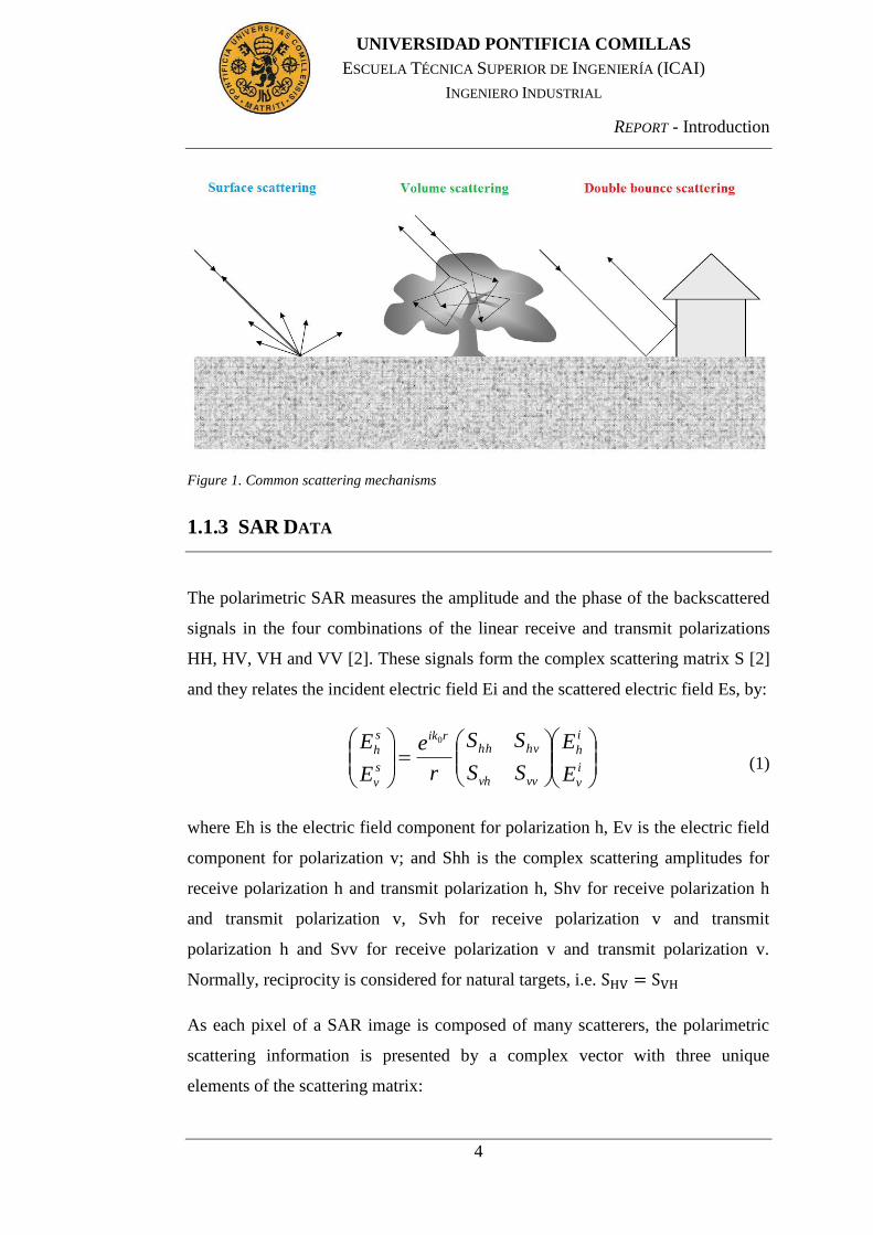
1.1.2 COMMON SCATTERING MECHANISMS
Figure 1 shows the three most common scattering mechanisms that occur in radar
remote sensing of the land surface.
The first mechanism is surface scattering in which the energy can be seen to
scatter or reflect from a well-defined interface.
The second is volume scattering, for which there is no identifiable single or
countable number of scattering sites; instead, the reflections are seen to come
from a myriad of scattering elements, such as the components of a tree canopy.
The third is called strong or hard target scattering and can come in a variety of
forms. The relevant one in this study is shown on Figure 1 as double bounce
scattering. [1]
REPORT - Introduction
4
UNIVERSIDAD PONTIFICIA COMILLAS
ESCUELA TÉCNICA SUPERIOR DE INGENIERÍA (ICAI)
INGENIERO INDUSTRIAL
Figure 1. Common scattering mechanisms
1.1.3 SAR DATA
The polarimetric SAR measures the amplitude and the phase of the backscattered
signals in the four combinations of the linear receive and transmit polarizations
HH, HV, VH and VV [2]. These signals form the complex scattering matrix S [2]
and they relates the incident electric field Ei and the scattered electric field Es, by:
i
v
i
h
vvvh
hvhhrik
s
v
s
h
E
E
SS
SS
r
e
E
E 0
(1)
where Eh is the electric field component for polarization h, Ev is the electric field
component for polarization v; and Shh is the complex scattering amplitudes for
receive polarization h and transmit polarization h, Shv for receive polarization h
and transmit polarization v, Svh for receive polarization v and transmit
polarization h and Svv for receive polarization v and transmit polarization v.
Normally, reciprocity is considered for natural targets, i.e.
As each pixel of a SAR image is composed of many scatterers, the polarimetric
scattering information is presented by a complex vector with three unique
elements of the scattering matrix:
REPORT - Introduction
5
UNIVERSIDAD PONTIFICIA COMILLAS
ESCUELA TÉCNICA SUPERIOR DE INGENIERÍA (ICAI)
INGENIERO INDUSTRIAL
(2)
The backscatter of the polarimetric covariance matrix can be considered as the
average of the covariance matrices of individual scatterers in each pixel. This
polarimetric covariance matrix for each pixel is defined as:
(3)
The decomposition of the covariance matrix in different types of reflection
simplifies the data, thus the surface features can be identified readily.
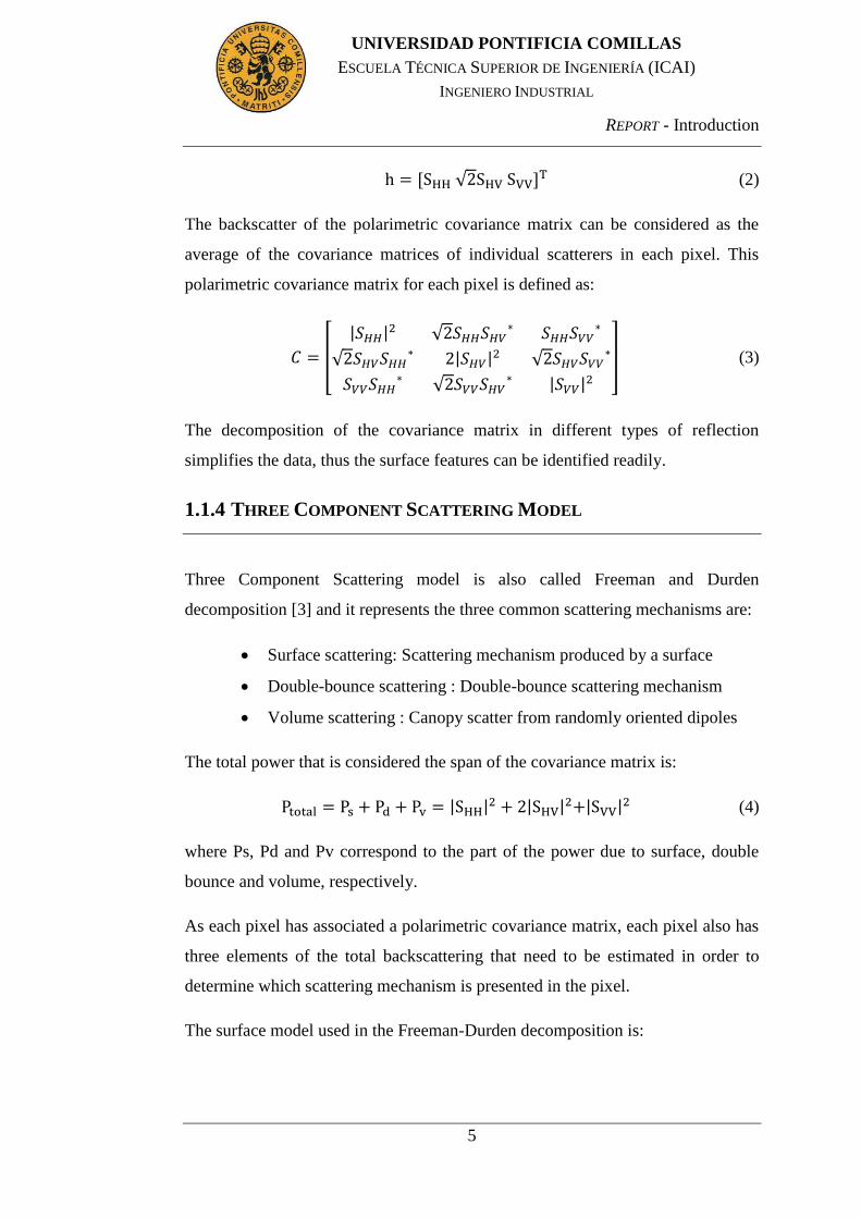
1.1.4 THREE COMPONENT SCATTERING MODEL
Three Component Scattering model is also called Freeman and Durden
decomposition [3] and it represents the three common scattering mechanisms are:
Surface scattering: Scattering mechanism produced by a surface
Double-bounce scattering : Double-bounce scattering mechanism
Volume scattering : Canopy scatter from randomly oriented dipoles
The total power that is considered the span of the covariance matrix is:
(4)
where Ps, Pd and Pv correspond to the part of the power due to surface, double
bounce and volume, respectively.
As each pixel has associated a polarimetric covariance matrix, each pixel also has
three elements of the total backscattering that need to be estimated in order to
determine which scattering mechanism is presented in the pixel.
The surface model used in the Freeman-Durden decomposition is:
REPORT - Introduction
6
UNIVERSIDAD PONTIFICIA COMILLAS
ESCUELA TÉCNICA SUPERIOR DE INGENIERÍA (ICAI)
INGENIERO INDUSTRIAL
10
000
0
10
000
0
103
1
03
20
3101
**
2
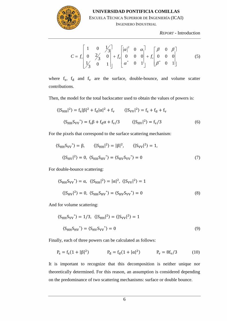
vdv fffC (5)
where , and are the surface, double-bounce, and volume scatter
contributions.
Then, the model for the total backscatter used to obtain the values of powers is:
(6)
For the pixels that correspond to the surface scattering mechanism:
(7)
For double-bounce scattering:
(8)
And for volume scattering:
(9)
Finally, each of three powers can be calculated as follows:
(10)
It is important to recognize that this decomposition is neither unique nor
theoretically determined. For this reason, an assumption is considered depending
on the predominance of two scattering mechanisms: surface or double bounce.

REPORT - Introduction
7
UNIVERSIDAD PONTIFICIA COMILLAS
ESCUELA TÉCNICA SUPERIOR DE INGENIERÍA (ICAI)
INGENIERO INDUSTRIAL
If surface scattering mechanism is dominant, it is assumed that
and , and in order to solve the equation system, the parameter
“α” is set to -1. On the other hand, if , the double-bounce
scattering mechanism is dominant and the parameter “β” is set to 1.
1.1.5 ENTROPY BASED SCATTERING MODEL
Entropy based model, also called Cloude and Pottier decomposition, propose an
algorithm [4] [5] composed of an unsupervised target decomposition classifier.
In this model, the covariance matrix is converted to a coherency matrix by a linear
transform:
(11)
where:
(12)
Then, applying eigenvalue analysis, the multilook coherency matrix is
decomposed as:
(13)
where λ1, λ2 and λ3 are the eigenvalues of the coherency matrix and e1, e2 and e3
their eigenvectors. Furthermore, the eigenvectors can be written as:
(14)
The average of angle that corresponds to the type of scatterers and varies from 0
to 90 degrees:
(15)
TTTeeeeeeT
*
333
*
222
*
111
Ti
ii
i
iii
i
iiii eeee sinsincossincos
REPORT - Introduction
8
UNIVERSIDAD PONTIFICIA COMILLAS
ESCUELA TÉCNICA SUPERIOR DE INGENIERÍA (ICAI)
INGENIERO INDUSTRIAL
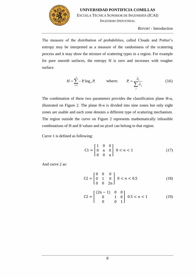
The measure of the distribution of probabilities, called Cloude and Pottier’s
entropy may be interpreted as a measure of the randomness of the scattering
process and it may show the mixture of scattering types in a region. For example
for pure smooth surfaces, the entropy H is zero and increases with rougher
surface.
3
1
3logi
ii PPH
j
j
iiP
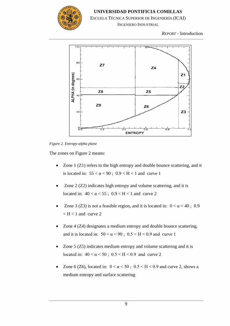
The combination of these two parameters provides the classification plane H-α,
illustrated on Figure 2. The plane H-α is divided into nine zones but only eight
zones are usable and each zone denotes a different type of scattering mechanism.
The region outside the curve on Figure 2 represents mathematically infeasible
combinations of H and values and no pixel can belong to that region.
Curve 1 is defined as following:
(17)
And curve 2 as:
(18)
(19)
REPORT - Introduction
9
UNIVERSIDAD PONTIFICIA COMILLAS
ESCUELA TÉCNICA SUPERIOR DE INGENIERÍA (ICAI)
INGENIERO INDUSTRIAL
Figure 2. Entropy-alpha plane
The zones on Figure 2 means:
Zone 1 (Z1) refers to the high entropy and double bounce scattering, and it
is located in: 55 < α < 90 ; 0.9 < H < 1 and curve 1
Zone 2 (Z2) indicates high entropy and volume scattering, and it is
located in: 40 < α < 55 ; 0.9 < H < 1 and curve 2
Zone 3 (Z3) is not a feasible region, and it is located in: 0 < α < 40 ; 0.9
< H < 1 and curve 2
Zone 4 (Z4) designates a medium entropy and double bounce scattering,
and it is located in: 50 < α < 90 ; 0.5 < H < 0.9 and curve 1
Zone 5 (Z5) indicates medium entropy and volume scattering and it is
located in: 40 < α < 50 ; 0.5 < H < 0.9 and curve 2
Zone 6 (Z6), located in: 0 < α < 50 ; 0.5 < H < 0.9 and curve 2, shows a
medium entropy and surface scattering
REPORT - Introduction
10
UNIVERSIDAD PONTIFICIA COMILLAS
ESCUELA TÉCNICA SUPERIOR DE INGENIERÍA (ICAI)
INGENIERO INDUSTRIAL
Zone 7 (Z7) designates a low entropy and double bounce scattering, and it
is located in: 47.5 < α < 90 and 0 < H < 0.5
Zone 8 (Z8) indicates low entropy and volume scattering, and it is located
in: 42.5 < α < 47.5 and 0 < H < 0.5
Zone 9 (Z9) is located in: 0 < α < 42.5 ; 0 < H < 0.5 and curve 2
1.1.6 SPECKLE IN SAR IMAGES
Speckle is one of the most serious disadvantages of SAR images. It is a coherent
interference of waves scattered from terrain elements observed in each resolution
cell (set of pixels).
The process of the coherent interference is the following; an incident radar wave
interacts with each element of the surface and surface cover to generate scattered
waves propagating in all directions. Those scattered waves that reach the
receiving antenna are summed in direction and phase to make the received signal.
The relative phase components contain the differential propagation paths.
The SAR focusing operation coherently combines the received signals to form the
image. Then, the scattered wave phase addition results in both constructive and
destructive interference of individual scattered returns and randomly modulates
the strength of the signal in each resolution cell. The constructive interference is
an increase from the mean intensity and produces bright pixels, and the
destructive interference is a decrease from the mean intensity and produces dark
pixels. Finally, these random fluctuations give rise to speckle. [6]
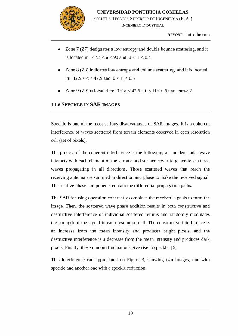
This interference can appreciated on Figure 3, showing two images, one with
speckle and another one with a speckle reduction.
REPORT - Introduction
11
UNIVERSIDAD PONTIFICIA COMILLAS
ESCUELA TÉCNICA SUPERIOR DE INGENIERÍA (ICAI)
INGENIERO INDUSTRIAL
Figure 3. SAR image with speckle at the left and the same image filtered reducing the speckle [7]
1.1.6.1 Speckle filter
Lee filter [8] was applied to reduce the speckle. It is a boxcar filter characterized
by avoiding the two main limitations of general boxcar filters:
sharp edges are generally blurred
point scatterers are over filtered and transformed to spread targets
The measure of speckle noise is determined as follows:
where N is a number of looks that can be estimated according to the variance to
ratio taken for several homogeneous areas. The equivalent number of looks can be
calculated as following:
(20)
REPORT - Introduction
12
UNIVERSIDAD PONTIFICIA COMILLAS
ESCUELA TÉCNICA SUPERIOR DE INGENIERÍA (ICAI)
INGENIERO INDUSTRIAL
where VMR denotes variance-to-mean-squared ratio and m is the multilook
image.
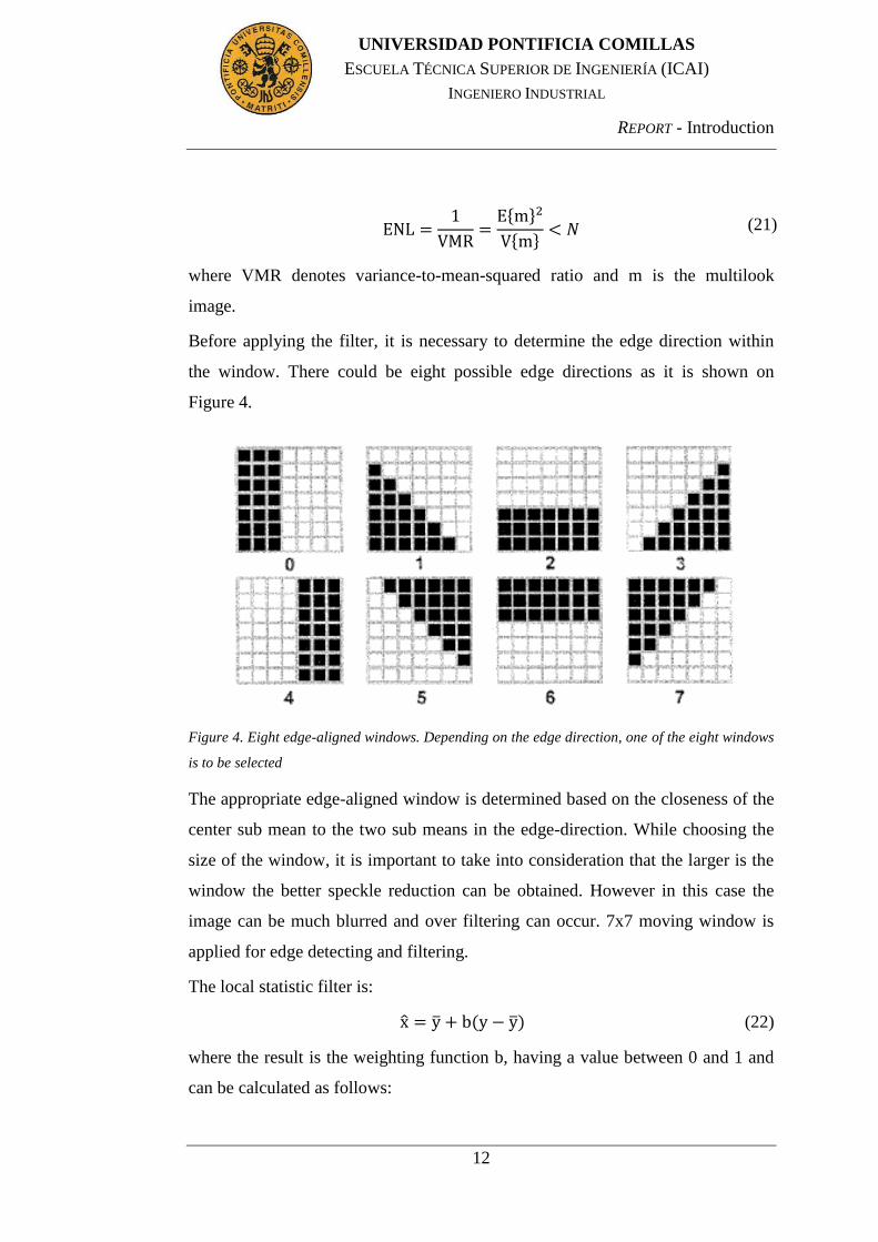
Before applying the filter, it is necessary to determine the edge direction within
the window. There could be eight possible edge directions as it is shown on
Figure 4.
Figure 4. Eight edge-aligned windows. Depending on the edge direction, one of the eight windows
is to be selected
The appropriate edge-aligned window is determined based on the closeness of the
center sub mean to the two sub means in the edge-direction. While choosing the
size of the window, it is important to take into consideration that the larger is the
window the better speckle reduction can be obtained. However in this case the
image can be much blurred and over filtering can occur. 7x7 moving window is
applied for edge detecting and filtering.
The local statistic filter is:
(22)
where the result is the weighting function b, having a value between 0 and 1 and
can be calculated as follows:
(21)

REPORT - Introduction
13
UNIVERSIDAD PONTIFICIA COMILLAS
ESCUELA TÉCNICA SUPERIOR DE INGENIERÍA (ICAI)
INGENIERO INDUSTRIAL
where is the local variance and is the variance of the reflectance
without speckle noise. For inhomogeneous areas is high. For
homogeneous are and .
The span image is used to compute the weight in a selected edge-aligned window.
Then, the weighting function and one of the eight edge aligned windows are used
to filter the whole covariance matrix, including the off-diagonal terms. The
filtered covariance matrix is:
(24)
where each element of is the local mean, computed with pixels in the same
edge-aligned window. It should be noted when applying the filter to a window,
may be negative due to insufficient samples or due to using larger than the
correct value of . If so, should be set to zero to ensure that the weight is
between zero and one.
1.2 MOTIVATION
One of the biggest challenges facing humanity is the understanding of the
environment, particularly with respect to land use and the conservation of natural
resources. Besides, due to global population growth makes the agricultural sector
a social and economic factor very essential. In recent decades, several and
significant changes in agricultural techniques have been generated primarily by
the need to increase crop production. Therefore, in order to make estimates of
agricultural production is also necessary to develop methods to monitor the status
of crops and its stage of development.
Remote sensing is a technique that has analyzed the classification of agricultural
crops and their monitorization for a long time. In particular, Synthetic Aperture
(23)

REPORT - Introduction
14
UNIVERSIDAD PONTIFICIA COMILLAS
ESCUELA TÉCNICA SUPERIOR DE INGENIERÍA (ICAI)
INGENIERO INDUSTRIAL
Radar (SAR) offers great advantages over the optical and infrared sensors for
agricultural applications. The ability to map the terrain is higher in different
weather situations, such as cloud cover. Moreover, the radar backscatter is
sensitive to the size, shape and form of vegetation, as well as its orientation and
surface roughness [9].
The test site used in this study is ideally suited for evaluation of the performance
of different algorithms for agriculture and land-cover mapping. Especially, the
1998 data set, with its monthly coverage of the area during the growing season is
well-suited for simulating the performance of satellite systems.
1.3 OBJECTIVES
The main aim of this report is to develop and implement two statistical methods
based on image interpretation of polarimetric SAR data, in order to monitor the
development and the mappping of crops.
The results can be combined with classification techniques and with models of
crop growth, to improve the individual classification of crops and their prediction.
According to this main aim, the objectives can resume as following:
Implementation in MATLAB of two decomposition statistical methods to
analyze SAR data:
o Three Component Scattering model
o Entropy Based Scattering model
Analysis and comparison of these two methods
Classification of the crops or seeds from SAR data of the test site used in
the study
Analysis and evaluation of the development of these crops
REPORT - Introduction
15
UNIVERSIDAD PONTIFICIA COMILLAS
ESCUELA TÉCNICA SUPERIOR DE INGENIERÍA (ICAI)
INGENIERO INDUSTRIAL
1.4 METHODOLOGY
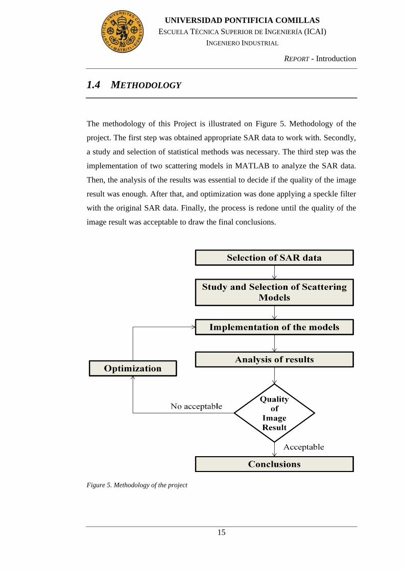
The methodology of this Project is illustrated on Figure 5. Methodology of the
project. The first step was obtained appropriate SAR data to work with. Secondly,
a study and selection of statistical methods was necessary. The third step was the
implementation of two scattering models in MATLAB to analyze the SAR data.
Then, the analysis of the results was essential to decide if the quality of the image
result was enough. After that, and optimization was done applying a speckle filter
with the original SAR data. Finally, the process is redone until the quality of the
image result was acceptable to draw the final conclusions.
Figure 5. Methodology of the project
REPORT - Introduction
16
UNIVERSIDAD PONTIFICIA COMILLAS
ESCUELA TÉCNICA SUPERIOR DE INGENIERÍA (ICAI)
INGENIERO INDUSTRIAL
1.5 SOURCES USED AND SUPPORTING TOOLS
1.5.1 TEST SITE
The Foulum test site is located at the Research Centre Foulum of the Danish
Institute of Agricultural Sciences, and it contains a large number of agricultural
fields with different crops, as well as several lakes, forests, areas with natural
vegetation, grasslands, and urban areas.
The area of plant production includes facilities for experimental cultivation as
well as research in applied cropping systems and specialized facilities. Research
Centre Foulum disposes of a built up area of approx. 100,000 m2 and 550 hectares
of land. The forest areas consist of deciduous forest and coniferous forest:
Norway spruce and Caucasian fir.
The crop types present in the area are 10, for spring crops: beets, peas, potatoes,
maize, spring barley, and oats, and for winter crops: rye, winter barley, winter
wheat, winter rape, and grass. However, the land area has 7 relevant types of
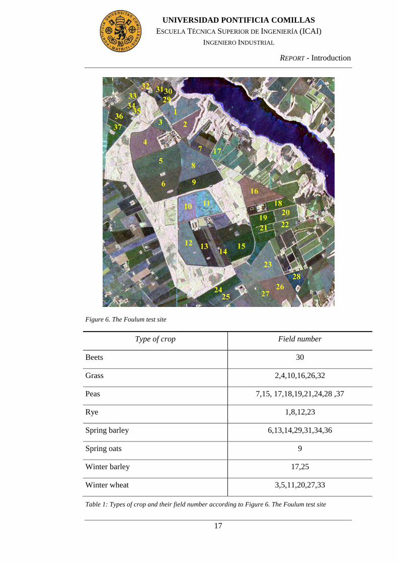
crops for this study and in total 37 fields of them, this is shown on Figure 6. This
area is relatively flat, and corrections of the local incidence angle due to terrain
slope are therefore as a first approximation not necessary.
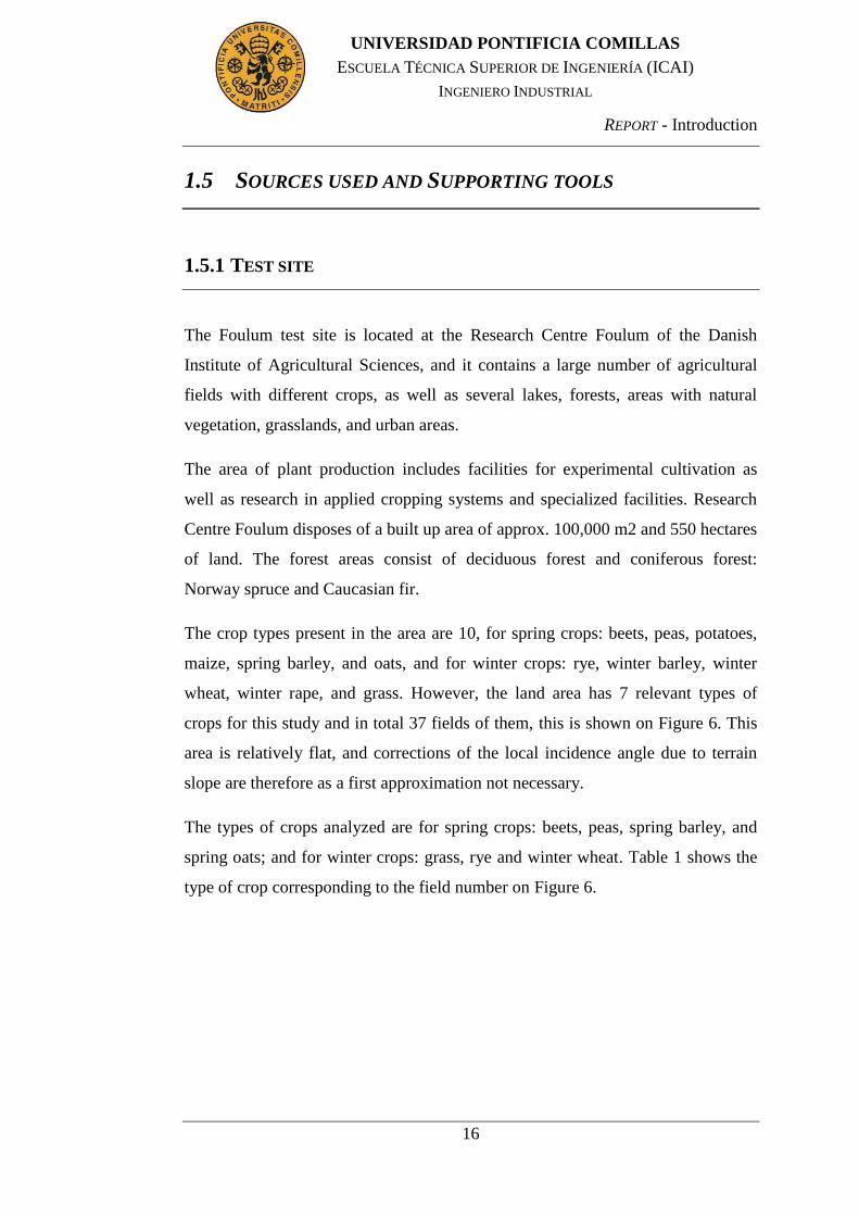
The types of crops analyzed are for spring crops: beets, peas, spring barley, and
spring oats; and for winter crops: grass, rye and winter wheat. Table 1 shows the
type of crop corresponding to the field number on Figure 6.
REPORT - Introduction
17
UNIVERSIDAD PONTIFICIA COMILLAS
ESCUELA TÉCNICA SUPERIOR DE INGENIERÍA (ICAI)
INGENIERO INDUSTRIAL
Figure 6. The Foulum test site
Type of crop Field number
Beets 30
Grass 2,4,10,16,26,32
Peas 7,15, 17,18,19,21,24,28 ,37
Rye 1,8,12,23
Spring barley 6,13,14,29,31,34,36
Spring oats 9
Winter barley 17,25
Winter wheat 3,5,11,20,27,33
Table 1: Types of crop and their field number according to Figure 6. The Foulum test site
REPORT - Introduction
18
UNIVERSIDAD PONTIFICIA COMILLAS
ESCUELA TÉCNICA SUPERIOR DE INGENIERÍA (ICAI)
INGENIERO INDUSTRIAL
1.5.2 DATA
The ability of SAR to penetrate cloud cover makes it particularly valuable in
frequently cloudy areas. Image data serve to map and monitor the use of the land,
and these data are of gaining importance for forestry and agriculture .
In this study, the SAR data were acquired by the fully polarimetric Danish
airborne SAR system, EMISAR, which operates at two frequencies, C-band (5.3
GHz/5.7 cm wavelength) and L-band (1.25 GHz/24 cm wavelength). The
nominal one-look spatial resolution is 2 m by 2 m (one-look); the ground range
swath is approximately 12 km and typical incidence angles range from 35º to 60º.
The processed data from this system are fully calibrated by using an advanced
internal calibration system. In the period from 1993 to 1999 the Foulum test site
has been covered by the EMISAR many times, because the test site has acted as
calibration site for the system. In 1998 simultaneous L-band and C-band data
were acquired over the Foulum agricultural test site in Jutland, Denmark, on 21
March, 17 April, 20 May, 16 June, 15 July and 16 August. On 17 April, 20 May,
16 June, and 15 July four parallel acquisitions were made with different incidence
angles. Each field was therefore measured with four different incidence angles,
with values ranging from about 20° to 65°.
All acquisitions were co-registered by identifying ground control points in the
images and using an interferometric DEM acquired by the EMISAR system.
Before resampling, the original one-look scattering matrix data were transformed
to covariance matrix data, and these data were averaged to reduce the speckle by a
cosine-squared weighted 9 by 9 filter. The new pixel spacing in the images is 5 m
by 5 m, and the effective spatial resolution is approximately 8 m by 8 m at mid-
range. After the averaging the equivalent number of looks is estimated to be 9-11
from homogenous areas in the images. This corresponds to a standard deviation
for the backscatter coefficient of approximately 1.1 – 1.8 dB.
REPORT - Introduction
19
UNIVERSIDAD PONTIFICIA COMILLAS
ESCUELA TÉCNICA SUPERIOR DE INGENIERÍA (ICAI)
INGENIERO INDUSTRIAL
1.5.3 PROGRAMMING LANGUAGE: MATLAB
MATLAB is a matrix processing language and images are represented as
matrices. Thus, instead of representing pixel positions as (x,y), it is common to
use the notation (r,c) indicating the row and column position of a pixel in the
matrix.
MATLAB provides an image input function, “imread()”, that reads an image from
a graphics file. The return value is an array containing the image data. If the file
contains a grayscale image, the return value is an M-by-N array. If the file
contains a truecolor image, the return value is an M-by-N-by-3 array. To display
image data, the function is “imshow()” and displays the image stored in the
graphics file. The file must contain an image that can be read by “imread” or
“dicomread”. “imshow” calls “imread” or “dicomread” to read the image from the
file, but does not store the image data in the MATLAB workspace. If the file
contains multiple images, imshow displays the first image in the file. [10]
In addition, it was necessary to use other MATLAB function in this project. Since
statistic methods are implemented to analyze the SAR data, the MATLAB user
guide about mathematics were used [11]. A basic MATLAB programming guide
can also be found in the section Part II.
REPORT - Implementation
20
UNIVERSIDAD PONTIFICIA COMILLAS
ESCUELA TÉCNICA SUPERIOR DE INGENIERÍA (ICAI)
INGENIERO INDUSTRIAL
Chapter 2 IMPLEMENTATION
2.1 SPECKLE FILTER
Before applying the filter it is important to estimate the number of looks correctly
to obtain the value σ2 for the variance of the noise, σ is a measure of speckle
noise.
Equivalent number of looks can be determined as follows:
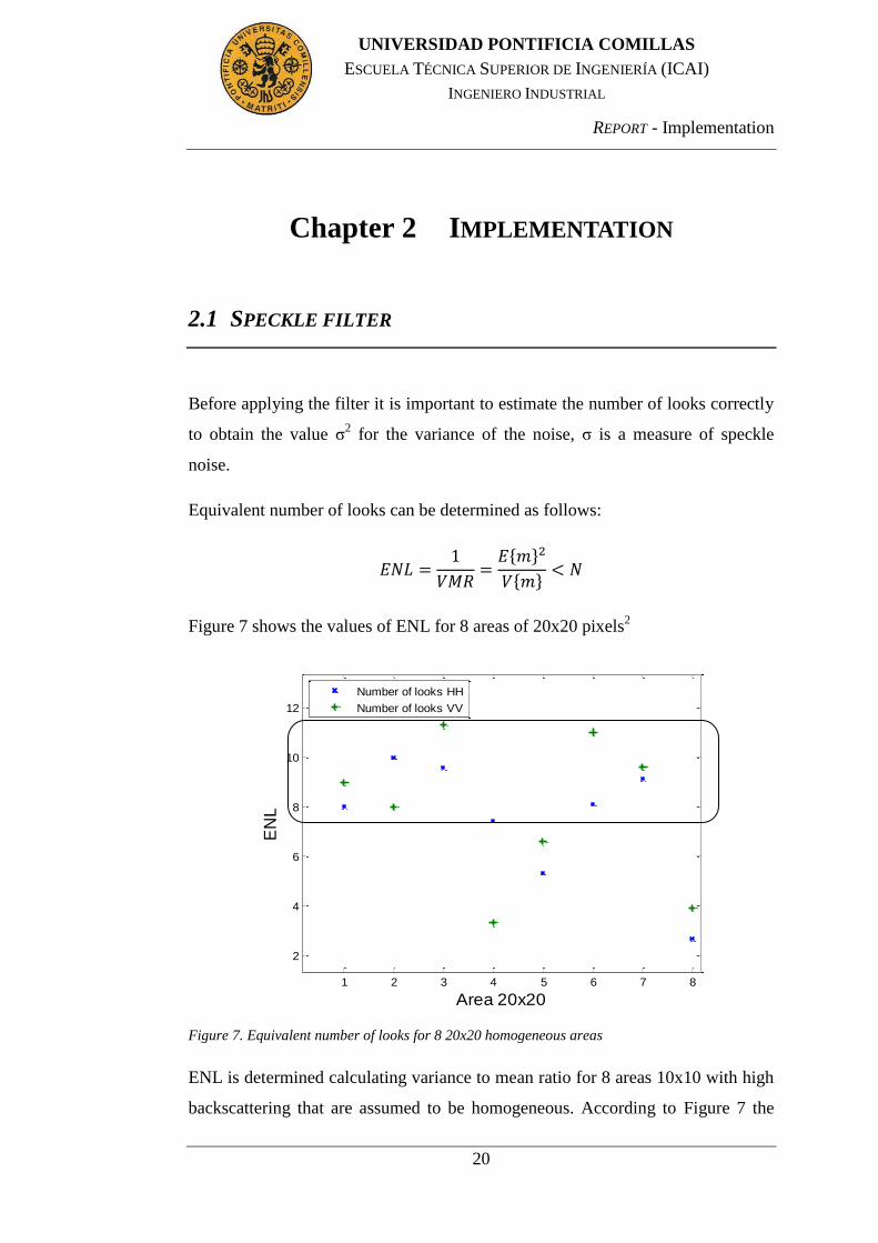
Figure 7 shows the values of ENL for 8 areas of 20x20 pixels2
Figure 7. Equivalent number of looks for 8 20x20 homogeneous areas
ENL is determined calculating variance to mean ratio for 8 areas 10x10 with high
backscattering that are assumed to be homogeneous. According to Figure 7 the
1 2 3 4 5 6 7 8
2
4
6
8
10
12
Area 20x20
EN
L
Number of looks HH
Number of looks VV
REPORT - Implementation
21
UNIVERSIDAD PONTIFICIA COMILLAS
ESCUELA TÉCNICA SUPERIOR DE INGENIERÍA (ICAI)
INGENIERO INDUSTRIAL
most plausible number of looks is 10 as for the most of the areas ENL is less than
10. Small values of ENL indicates that the variance of the values of and
are very large. This is possible because the image has a lot of speckle or
because the chosen area was not totally homogeneous.
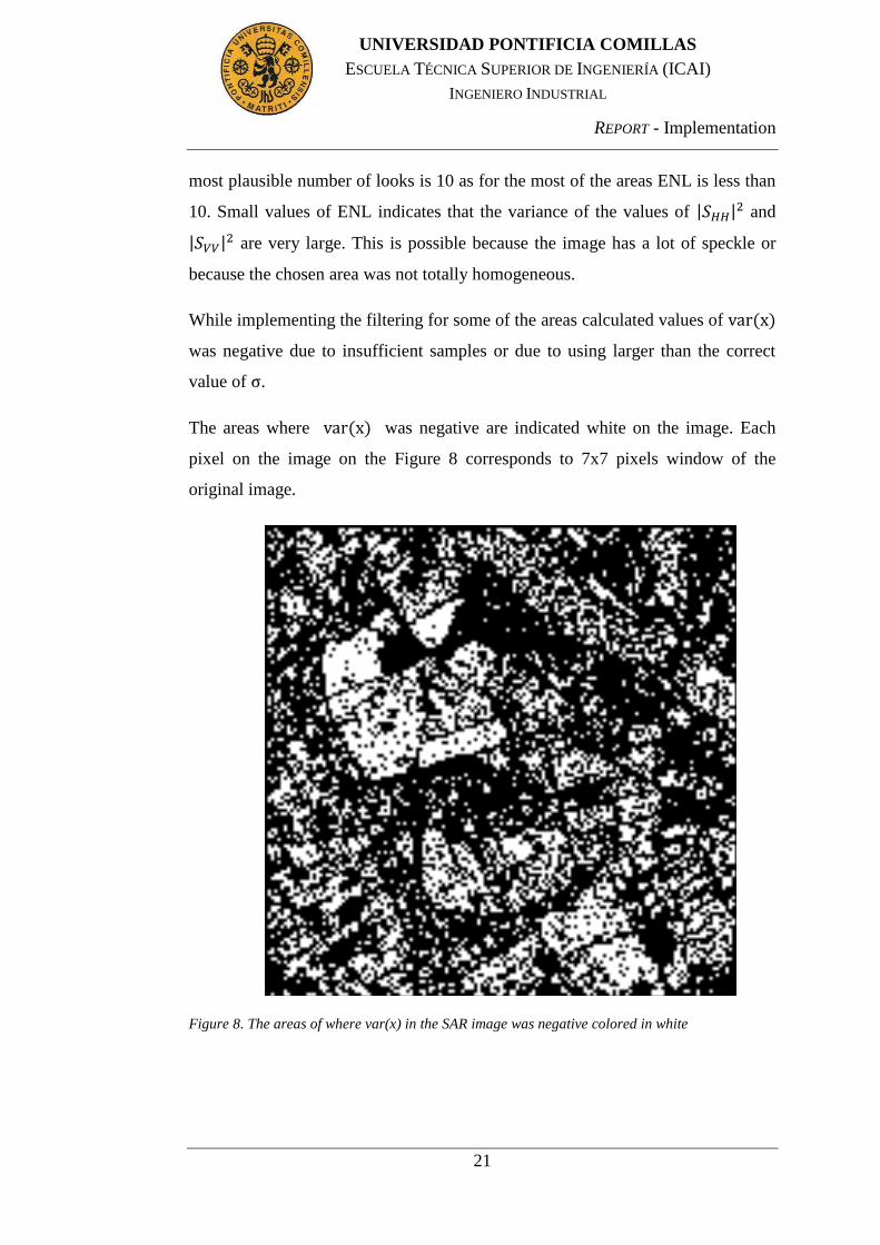
While implementing the filtering for some of the areas calculated values of
was negative due to insufficient samples or due to using larger than the correct
value of .
The areas where was negative are indicated white on the image. Each
pixel on the image on the Figure 8 corresponds to 7x7 pixels window of the
original image.
Figure 8. The areas of where var(x) in the SAR image was negative colored in white
REPORT - Implementation
22
UNIVERSIDAD PONTIFICIA COMILLAS
ESCUELA TÉCNICA SUPERIOR DE INGENIERÍA (ICAI)
INGENIERO INDUSTRIAL
2.2 THREE COMPONENT SCATTERING MODEL
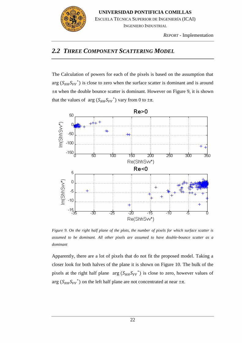
The Calculation of powers for each of the pixels is based on the assumption that
is close to zero when the surface scatter is dominant and is around
±π when the double bounce scatter is dominant. However on Figure 9, it is shown
that the values of vary from 0 to ±π.
Figure 9. On the right half plane of the plots, the number of pixels for which surface scatter is
assumed to be dominant. All other pixels are assumed to have double-bounce scatter as a
dominant
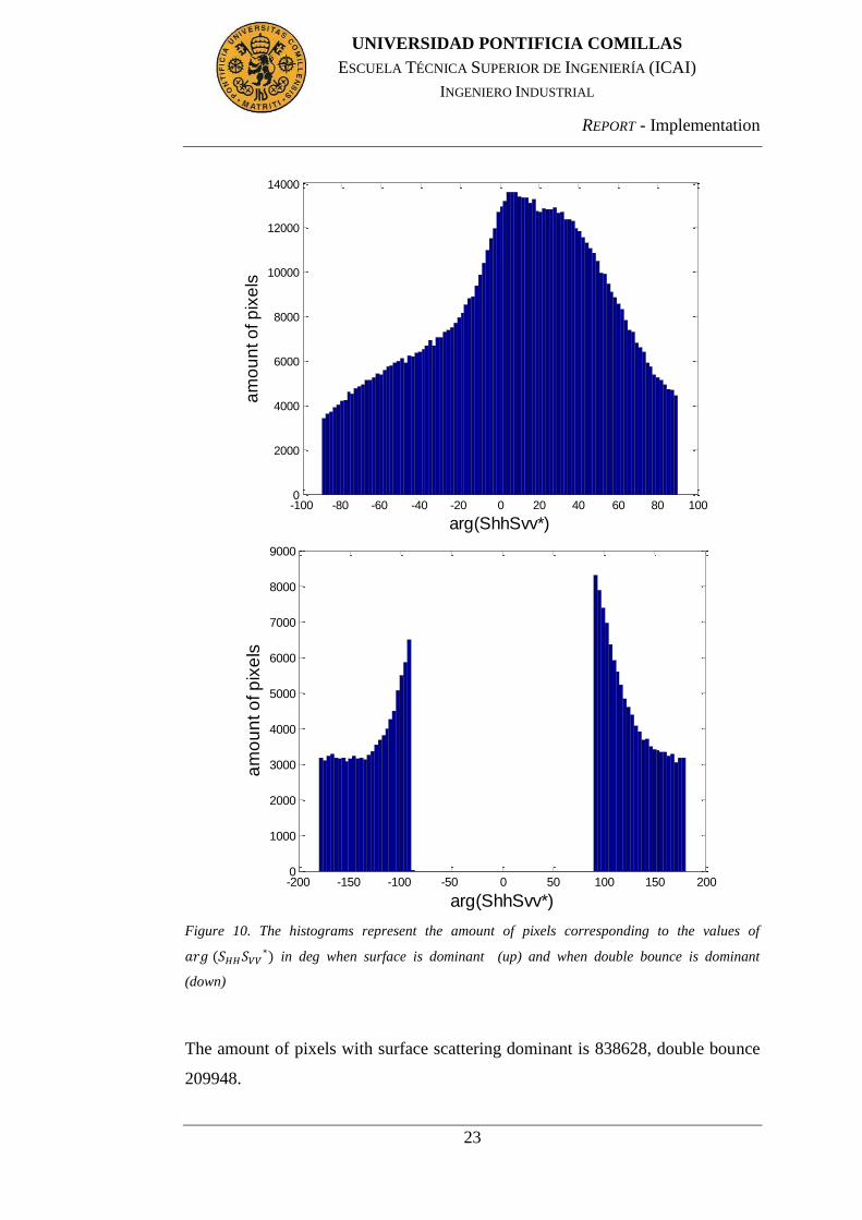
Apparently, there are a lot of pixels that do not fit the proposed model. Taking a
closer look for both halves of the plane it is shown on Figure 10. The bulk of the
pixels at the right half plane is close to zero, however values of
on the left half plane are not concentrated at near ±π.
REPORT - Implementation
23
UNIVERSIDAD PONTIFICIA COMILLAS
ESCUELA TÉCNICA SUPERIOR DE INGENIERÍA (ICAI)
INGENIERO INDUSTRIAL
Figure 10. The histograms represent the amount of pixels corresponding to the values of
in deg when surface is dominant (up) and when double bounce is dominant
(down)
The amount of pixels with surface scattering dominant is 838628, double bounce
209948.
-100 -80 -60 -40 -20 0 20 40 60 80 1000
2000
4000
6000
8000
10000
12000
14000
am
ou
nt o
f p
ixe
ls
arg(ShhSvv*)
-200 -150 -100 -50 0 50 100 150 2000
1000
2000
3000
4000
5000
6000
7000
8000
9000
am
ou
nt o
f p
ixe
ls
arg(ShhSvv*)
REPORT - Implementation
24
UNIVERSIDAD PONTIFICIA COMILLAS
ESCUELA TÉCNICA SUPERIOR DE INGENIERÍA (ICAI)
INGENIERO INDUSTRIAL
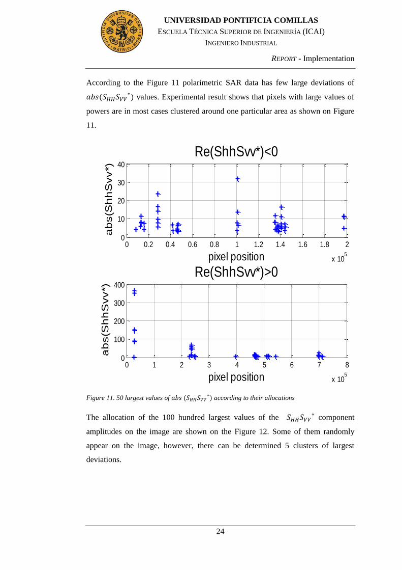
According to the Figure 11 polarimetric SAR data has few large deviations of
values. Experimental result shows that pixels with large values of
powers are in most cases clustered around one particular area as shown on Figure
11.
Figure 11. 50 largest values of according to their allocations
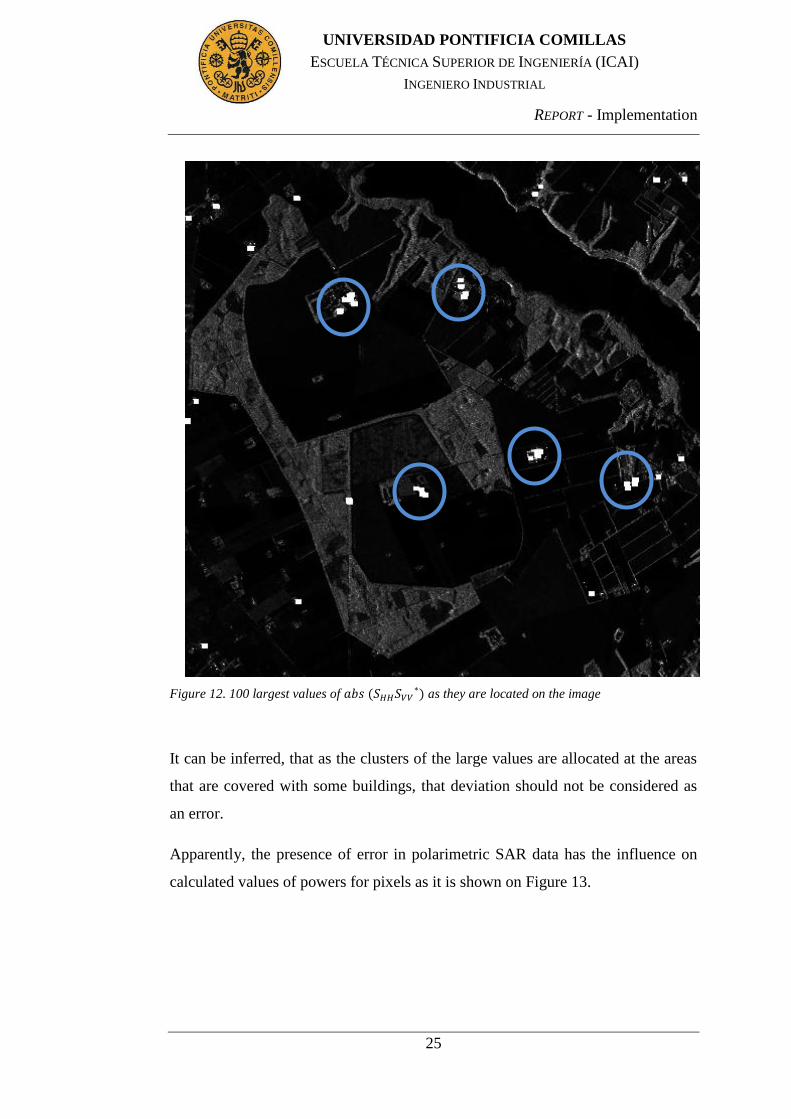
The allocation of the 100 hundred largest values of the component
amplitudes on the image are shown on the Figure 12. Some of them randomly
appear on the image, however, there can be determined 5 clusters of largest
deviations.
0 0.2 0.4 0.6 0.8 1 1.2 1.4 1.6 1.8 2
x 105
0
10
20
30
40
ab
s(S
hh
Svv*)
pixel position
Re(ShhSvv*)<0
0 1 2 3 4 5 6 7 8
x 105
0
100
200
300
400
ab
s(S
hh
Svv*)
pixel position
Re(ShhSvv*)>0
REPORT - Implementation
25
UNIVERSIDAD PONTIFICIA COMILLAS
ESCUELA TÉCNICA SUPERIOR DE INGENIERÍA (ICAI)
INGENIERO INDUSTRIAL
Figure 12. 100 largest values of as they are located on the image
It can be inferred, that as the clusters of the large values are allocated at the areas
that are covered with some buildings, that deviation should not be considered as
an error.
Apparently, the presence of error in polarimetric SAR data has the influence on
calculated values of powers for pixels as it is shown on Figure 13.
REPORT - Implementation
26
UNIVERSIDAD PONTIFICIA COMILLAS
ESCUELA TÉCNICA SUPERIOR DE INGENIERÍA (ICAI)
INGENIERO INDUSTRIAL
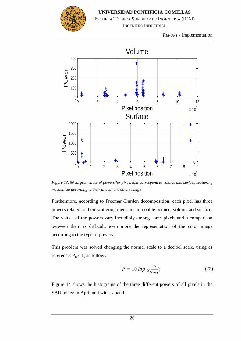
Figure 13. 50 largest values of powers for pixels that correspond to volume and surface scattering
mechanism according to their allocations on the image
Furthermore, according to Freeman-Durden decomposition, each pixel has three
powers related to their scattering mechanism: double bounce, volume and surface.
The values of the powers vary incredibly among some pixels and a comparison
between them is difficult, even more the representation of the color image
according to the type of powers.
This problem was solved changing the normal scale to a decibel scale, using as
reference: Pref=1, as follows:
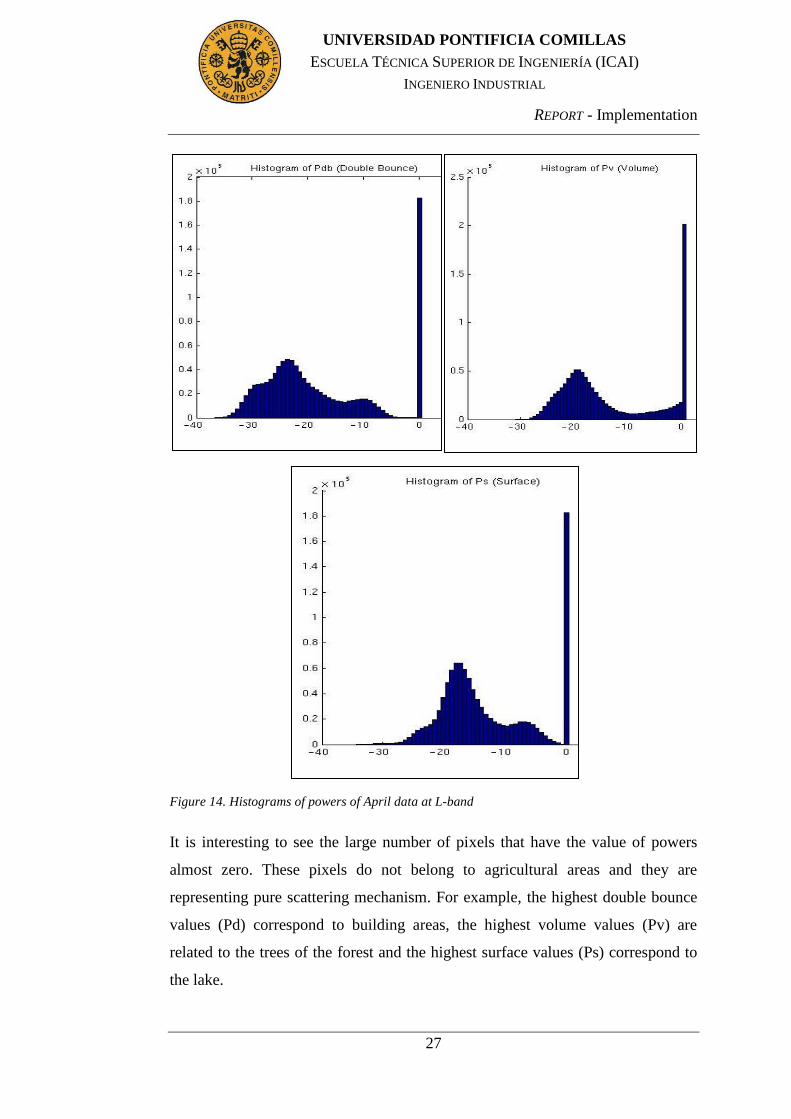
Figure 14 shows the histograms of the three different powers of all pixels in the
SAR image in April and with L-band.
0 2 4 6 8 10 12
x 105
0
100
200
300
400
Po
we
r
Pixel position
Volume
0 1 2 3 4 5 6 7 8 9
x 105
0
500
1000
1500
2000
Po
we
r
Pixel position
Surface
(25)
REPORT - Implementation
27
UNIVERSIDAD PONTIFICIA COMILLAS
ESCUELA TÉCNICA SUPERIOR DE INGENIERÍA (ICAI)
INGENIERO INDUSTRIAL
Figure 14. Histograms of powers of April data at L-band
It is interesting to see the large number of pixels that have the value of powers
almost zero. These pixels do not belong to agricultural areas and they are
representing pure scattering mechanism. For example, the highest double bounce
values (Pd) correspond to building areas, the highest volume values (Pv) are
related to the trees of the forest and the highest surface values (Ps) correspond to
the lake.
REPORT - Implementation
28
UNIVERSIDAD PONTIFICIA COMILLAS
ESCUELA TÉCNICA SUPERIOR DE INGENIERÍA (ICAI)
INGENIERO INDUSTRIAL
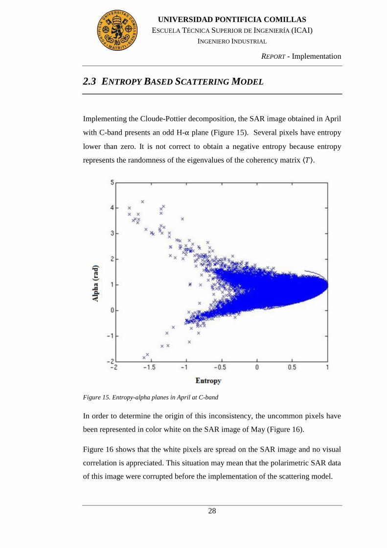
2.3 ENTROPY BASED SCATTERING MODEL
Implementing the Cloude-Pottier decomposition, the SAR image obtained in April
with C-band presents an odd H-α plane (Figure 15). Several pixels have entropy
lower than zero. It is not correct to obtain a negative entropy because entropy
represents the randomness of the eigenvalues of the coherency matrix .
Figure 15. Entropy-alpha planes in April at C-band
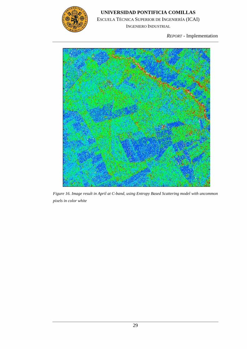
In order to determine the origin of this inconsistency, the uncommon pixels have
been represented in color white on the SAR image of May (Figure 16).
Figure 16 shows that the white pixels are spread on the SAR image and no visual
correlation is appreciated. This situation may mean that the polarimetric SAR data
of this image were corrupted before the implementation of the scattering model.
REPORT - Implementation
29
UNIVERSIDAD PONTIFICIA COMILLAS
ESCUELA TÉCNICA SUPERIOR DE INGENIERÍA (ICAI)
INGENIERO INDUSTRIAL
Figure 16. Image result in April at C-band, using Entropy Based Scattering model with uncommon
pixels in color white

REPORT - Results
30
UNIVERSIDAD PONTIFICIA COMILLAS
ESCUELA TÉCNICA SUPERIOR DE INGENIERÍA (ICAI)
INGENIERO INDUSTRIAL
Chapter 3 RESULTS
3.1 SPECKLE FILTER
The ideal situation is when the image would be colored just in black and white
after apply the filter, because in this case is close to 0 and ±π
values as it is assumed when applying the classification method.
The results indicate that the speckle is clearly reduced, however the image is still
much noisy. One of the reasons is that, while applying the filter, one of the eight
edge aligned windows was used in a moving 7x7 window, the situation when
there is no edge inside the window was not taken into consideration.
In the case where the window without edges is considered, it would be possible to
observe each field with only one color. Nevertheless, in some fields there are
buildings that produce small zones (very few amount of pixels) inside the fields
and it may be misunderstanding by noise.
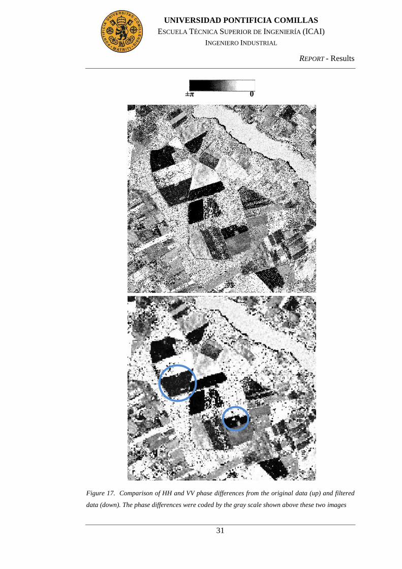
After filtering the amount of gray colored areas is reduced that indicates that HH
VV phase difference is more concentrated around the desired values. The results
of division into three categories (black, grey and white) before and after filtering
are shown on the Figure 17. Besides, two relevant fields with buildings areas are
marked with blue circles in the filtered image. The crops of the fields are black
and the buildings are represented by the color white.
REPORT - Results
31
UNIVERSIDAD PONTIFICIA COMILLAS
ESCUELA TÉCNICA SUPERIOR DE INGENIERÍA (ICAI)
INGENIERO INDUSTRIAL
Figure 17. Comparison of HH and VV phase differences from the original data (up) and filtered
data (down). The phase differences were coded by the gray scale shown above these two images
±π 0
REPORT - Results
32
UNIVERSIDAD PONTIFICIA COMILLAS
ESCUELA TÉCNICA SUPERIOR DE INGENIERÍA (ICAI)
INGENIERO INDUSTRIAL
3.2 THREE COMPONENT SCATTERING MODEL
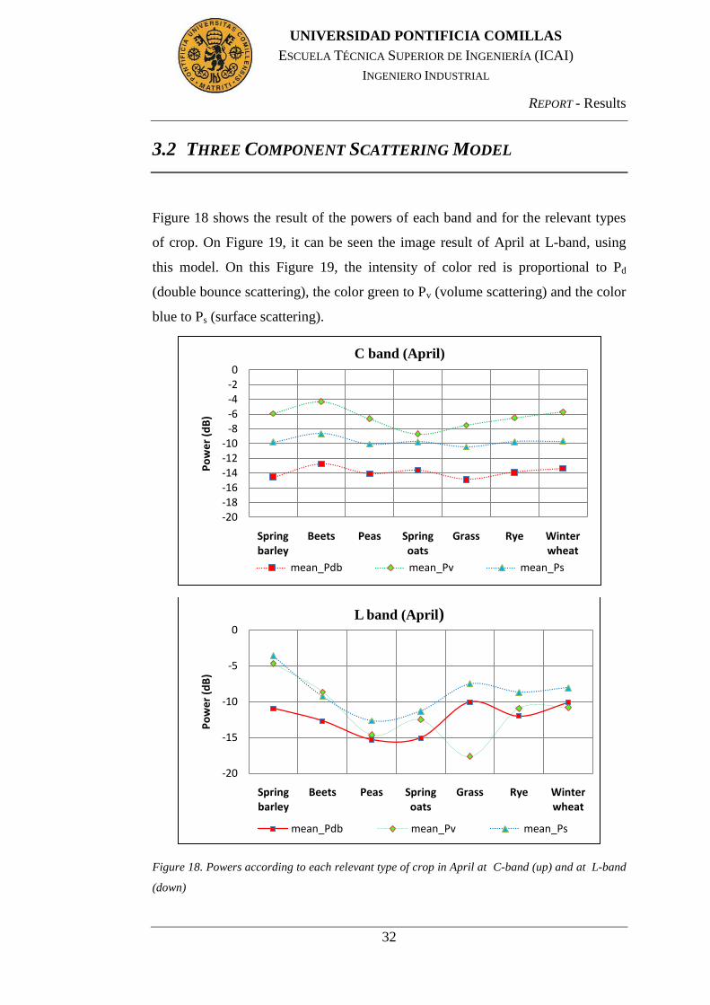
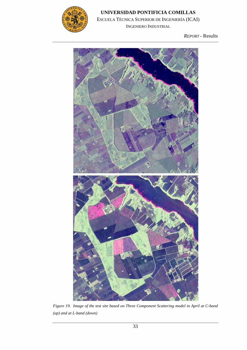
Figure 18 shows the result of the powers of each band and for the relevant types
of crop. On Figure 19, it can be seen the image result of April at L-band, using
this model. On this Figure 19, the intensity of color red is proportional to Pd
(double bounce scattering), the color green to Pv (volume scattering) and the color
blue to Ps (surface scattering).
Figure 18. Powers according to each relevant type of crop in April at C-band (up) and at L-band
(down)
-20-18-16-14-12-10
-8-6-4-20
Spring barley
Beets Peas Spring oats
Grass Rye Winter wheat
Po
we
r (d
B)
C band (April)
mean_Pdb mean_Pv mean_Ps
-20
-15
-10
-5
0
Spring barley
Beets Peas Spring oats
Grass Rye Winter wheat
Po
we
r (d
B)
L band (April)
mean_Pdb mean_Pv mean_Ps
REPORT - Results
33
UNIVERSIDAD PONTIFICIA COMILLAS
ESCUELA TÉCNICA SUPERIOR DE INGENIERÍA (ICAI)
INGENIERO INDUSTRIAL
Figure 19. Image of the test site based on Three Component Scattering model in April at C-band
(up) and at L-band (down)

REPORT - Results
34
UNIVERSIDAD PONTIFICIA COMILLAS
ESCUELA TÉCNICA SUPERIOR DE INGENIERÍA (ICAI)
INGENIERO INDUSTRIAL
SAR data corresponding in April was used in this section to analyze the different
types of crops because the height of each crop is significant in April. Grass (field
5) is very appreciable on the graphic of L-band (Figure 18). It has a high Ps and
Pd scattering and low Pv compared to other relevant crops. This is the reason that
grass is shown in color pink on Figure 19 spring barley (field 6, 13 and 14) spring
oats (field 9) and Peas has a higher Ps than Pd and Pv, this is shown in the dark
blue of these fields shown on the L-band of Figure 18. Beets (field 30) has a
higher Ps and Pv than Pd but Pv is higher than Ps, shown greener than other
mentioned fields at the L-band of Figure 19.
On the other hand, rye and winter wheat fields have the three powers very
similar, especially Pd and Pv, this is shown at both L-band and C- band on Figure
18. These both types of crops present the same color due to the similarity of the
crop plant and its development. C-band presents a higher Pv in all of the analyzed
fields due to the penetration of the wavelength.
The classification of crops must start assigning a specific class to each pixel. A
primary classification consists in defining three different classes according to each
power (Pd, Pv, Ps). Then, it is possible to divide each class in clusters in order to
obtain a more precise classification.
The difference between only 3 classes without clusters and the 15 clusters for
each class is shown on Figure 20; now using the May acquisition, because this
acquisition is more adequate to distinguish fields. The result of Figure 20 is
different of Figure 19 because Three Component Scattering model requires giving
the value of the highest power in each pixel, instead the value of the three of them.
Grass and winter wheat fields are clearly different compared to the other fields,
presenting a darker red. Besides, spring oats field shows a color practically
orange, differing from the rest of fields. In addition, peas and beets fields are
represented with dark blue and in this way they can distinguish from other fields
with the same surface scattering, such as rye field which presents a lighter blue.
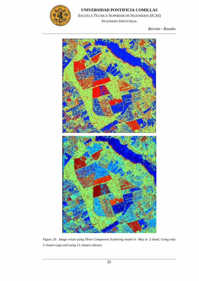
REPORT - Results
35
UNIVERSIDAD PONTIFICIA COMILLAS
ESCUELA TÉCNICA SUPERIOR DE INGENIERÍA (ICAI)
INGENIERO INDUSTRIAL
Figure 20. Image result using Three Component Scattering model in May at L-band. Using only
3 clusters (up) and using 15 clusters (down)

REPORT - Results
36
UNIVERSIDAD PONTIFICIA COMILLAS
ESCUELA TÉCNICA SUPERIOR DE INGENIERÍA (ICAI)
INGENIERO INDUSTRIAL
3.3 ENTROPY BASED SCATTERING MODEL
3.3.1 ENTROPY-ALPHA PLANES
The Foulum test site has several types of fields, including small buildings areas
forests and crops. The entropy based scattering provides a useful tool to classify
these terrains, H-α plane.
The April acquisition was not appropriate in this model because after the
implementation of the model, some pixels were placed outside the feasible
regions; this indicates inaccuracy in the SAR data used.
On Figure 21, there are two H-α planes corresponding to C and L band in May.
The results of this month are the most interesting because of the growth stage of
some of the crops.
The H-α planes in May shows that L-band has larger number of pixels with
double bounce scattering (zones 1, 4 y 7) and smooth surfaces, this is low entropy
and low alpha (zone 9) at L-band compared to C-band. This difference between
bands is because the penetration of the C-band is shorter than L-band.
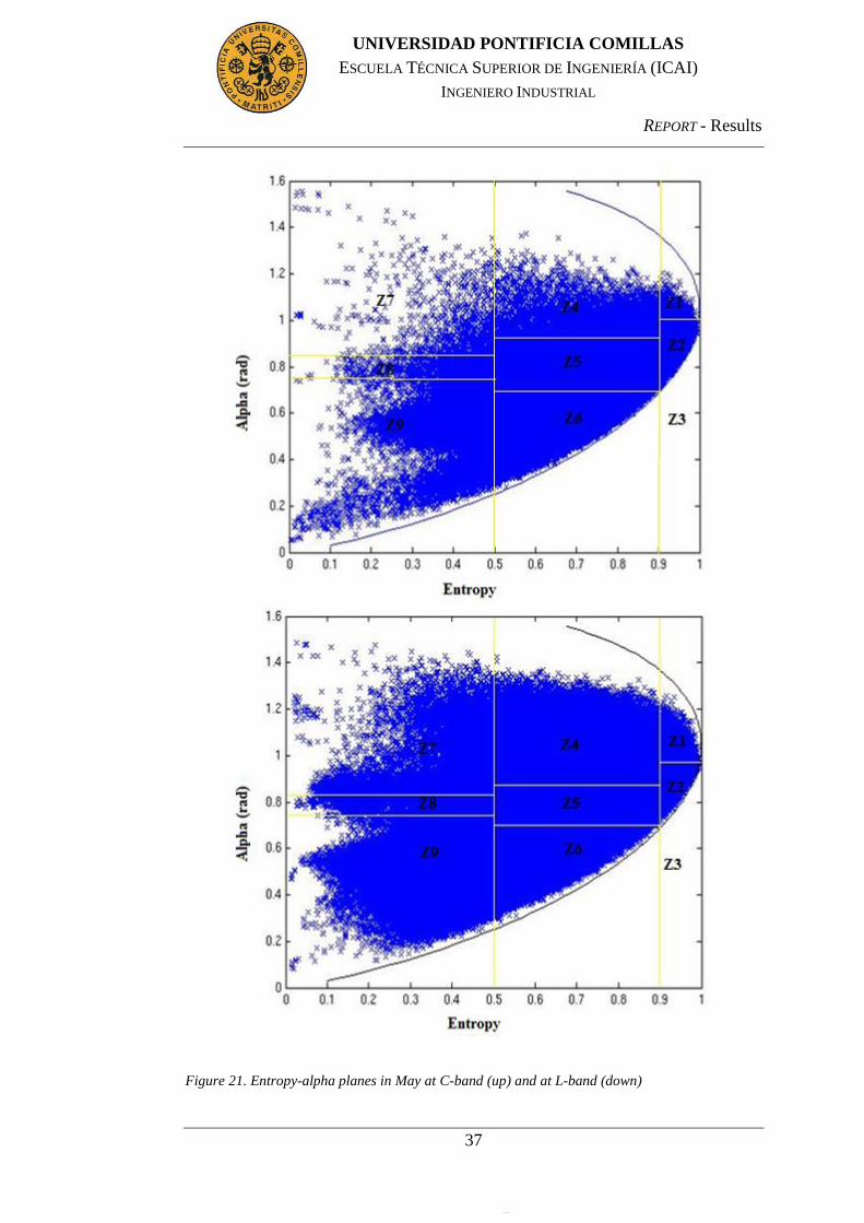
REPORT - Results
37
UNIVERSIDAD PONTIFICIA COMILLAS
ESCUELA TÉCNICA SUPERIOR DE INGENIERÍA (ICAI)
INGENIERO INDUSTRIAL
Figure 21. Entropy-alpha planes in May at C-band (up) and at L-band (down)

REPORT - Results
38
UNIVERSIDAD PONTIFICIA COMILLAS
ESCUELA TÉCNICA SUPERIOR DE INGENIERÍA (ICAI)
INGENIERO INDUSTRIAL
3.3.2 CLASSIFICATION OF CROPS
As it was mention in the previous section, the analysis of different types of crops
with this model was using the May acquisition, due to the inadequate SAR data in
April with C-band.
Grass (field 5) can be distinguished in both bands, but especially at C-band, where
its entropy has the lowest value. Spring barley (field 6, 13 and 14) shows the
highest entropy and alpha of the crops, this means that these spring barley fields
are roughness surfaces. Beets (field 30) and Pea fields have a higher value of
entropy when it was measured at L-band but the value of alpha almost remains
constant at L and C-band. rye and winter wheat fields are cereal very similar, that
is the reason because the entropy and alpha almost the same in both bands.
It can be inferred from the results on Figure 22 that cereals (spring barley, spring
oats, rye and winter wheat) have very similar scattering at C-band, both because
of entropy and alpha values, so they can distinguish between no cereal crops.
Moreover, it is possible to distinguish between them using the results of L-band,
but only spring cereals and winter cereals. The winter cereals, rye and winter
wheat, are always crops difficult to distinguish between them because they have
the same growth stage and very similar shape of plants.
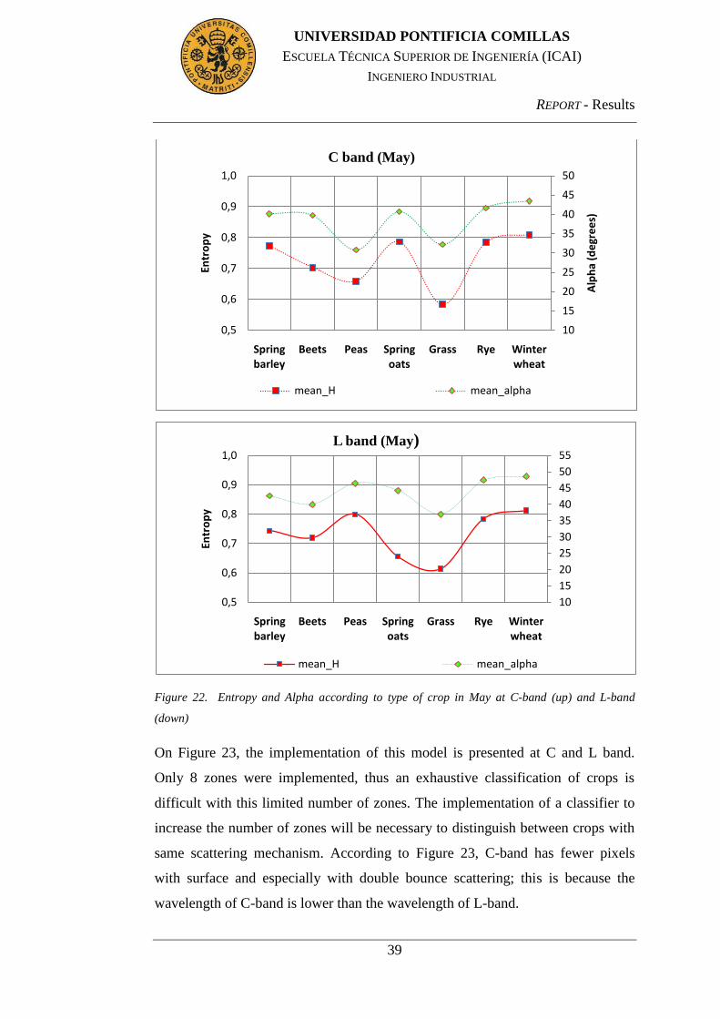
REPORT - Results
39
UNIVERSIDAD PONTIFICIA COMILLAS
ESCUELA TÉCNICA SUPERIOR DE INGENIERÍA (ICAI)
INGENIERO INDUSTRIAL
Figure 22. Entropy and Alpha according to type of crop in May at C-band (up) and L-band
(down)
On Figure 23, the implementation of this model is presented at C and L band.
Only 8 zones were implemented, thus an exhaustive classification of crops is
difficult with this limited number of zones. The implementation of a classifier to
increase the number of zones will be necessary to distinguish between crops with
same scattering mechanism. According to Figure 23, C-band has fewer pixels
with surface and especially with double bounce scattering; this is because the
wavelength of C-band is lower than the wavelength of L-band.
10
15
20
25
30
35
40
45
50
0,5
0,6
0,7
0,8
0,9
1,0
Spring barley
Beets Peas Spring oats
Grass Rye Winter wheat
Alp
ha
(de
gre
es)
Entr
op
y
C band (May)
mean_H mean_alpha
10
15
20
25
30
35
40
45
50
55
0,5
0,6
0,7
0,8
0,9
1,0
Spring barley
Beets Peas Spring oats
Grass Rye Winter wheat
Entr
op
y
L band (May)
mean_H mean_alpha
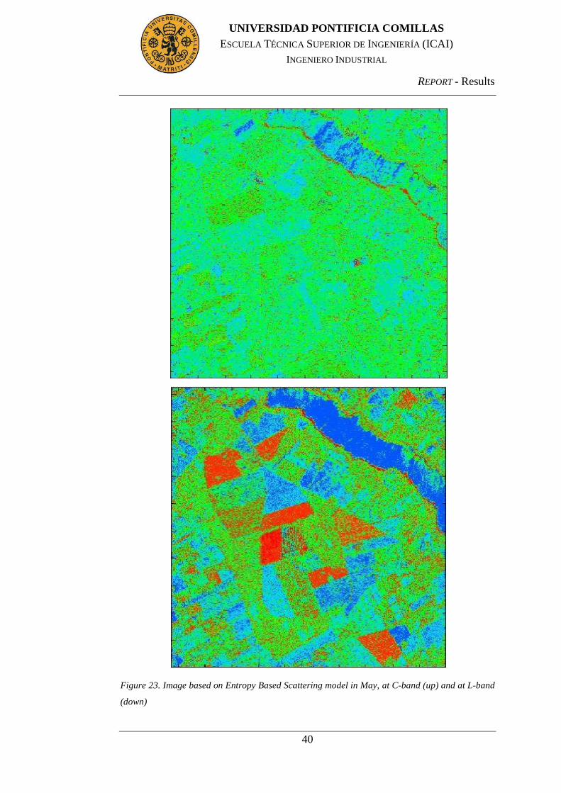
REPORT - Results
40
UNIVERSIDAD PONTIFICIA COMILLAS
ESCUELA TÉCNICA SUPERIOR DE INGENIERÍA (ICAI)
INGENIERO INDUSTRIAL
Figure 23. Image based on Entropy Based Scattering model in May, at C-band (up) and at L-band
(down)
REPORT - Results
41
UNIVERSIDAD PONTIFICIA COMILLAS
ESCUELA TÉCNICA SUPERIOR DE INGENIERÍA (ICAI)
INGENIERO INDUSTRIAL
3.4 COMPARISON OF MODELS
In this section, both scattering models are compared with and without filtering,
using the SAR data of May acquisition. This month is a crucial stage of all the
fields because spring and winter crops can be distinguished easily.
3.4.1 L-BAND
Figure 24 (a) and (b) show the results without filtering of the two models and they
are very similar. All the fields have speckle and in some of them the speckle is not
acceptable because it is not possible to recognize the field. However, Three
Component Scattering model seems to have more homogenous fields with almost
the same color for them. This occurs in fields 15, 19 and 21, all pea crops. For this
reason, it may infer that pea crops are more homogenous fields than others.
Furthermore, Three Component Scattering model presented on Figure 25 (a) has
better results after filtering, because can show different types of homogenous
fields with the same scattering. For instance, fields 18, 19, 21 and 24 are peas
crops and on Figure 25 (a) these are dark blue (surface), but on Figure 25(b), these
crops are not enough homogenous to consider the same type of crop although they
are measured as surface scattering too.
For double bounce, a similar situation happens. Fields 2, 4, 16 and 26 are grass. A
better displayed image results on Figure 25(a) than on Figure 25 (b). On the other
hand, two much details of surface scattering are gone in the huge area of volume
scattering on Figure 25 (a), this is not the case of Figure 25 (b).
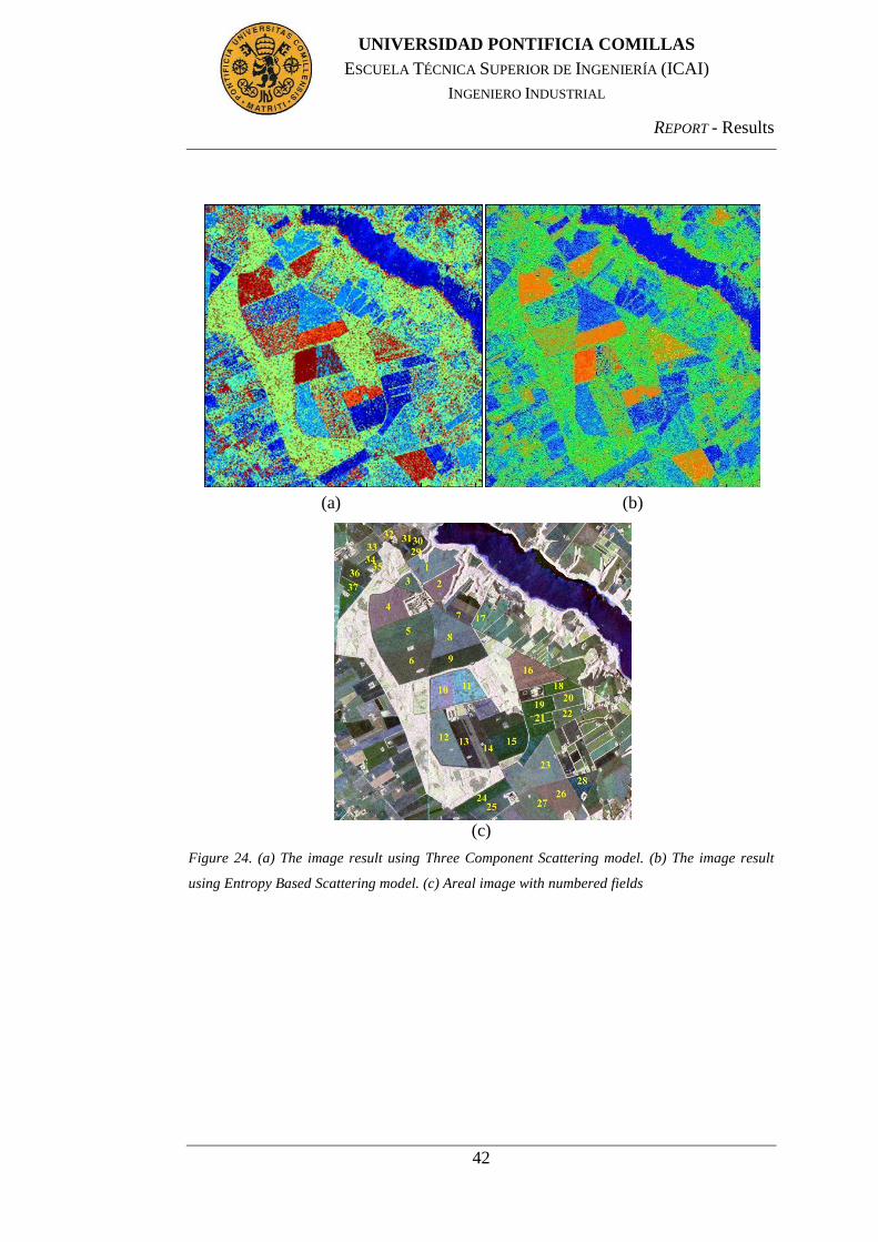
REPORT - Results
42
UNIVERSIDAD PONTIFICIA COMILLAS
ESCUELA TÉCNICA SUPERIOR DE INGENIERÍA (ICAI)
INGENIERO INDUSTRIAL
(a) (b)
(c)
Figure 24. (a) The image result using Three Component Scattering model. (b) The image result
using Entropy Based Scattering model. (c) Areal image with numbered fields
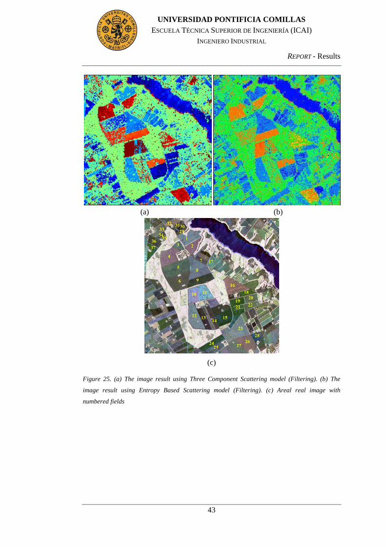
REPORT - Results
43
UNIVERSIDAD PONTIFICIA COMILLAS
ESCUELA TÉCNICA SUPERIOR DE INGENIERÍA (ICAI)
INGENIERO INDUSTRIAL
(a) (b)
(c)
Figure 25. (a) The image result using Three Component Scattering model (Filtering). (b) The
image result using Entropy Based Scattering model (Filtering). (c) Areal real image with
numbered fields

REPORT - Results
44
UNIVERSIDAD PONTIFICIA COMILLAS
ESCUELA TÉCNICA SUPERIOR DE INGENIERÍA (ICAI)
INGENIERO INDUSTRIAL
3.4.2 C-BAND
The models were also applied to the C-band of the data that was taken in different
periods of the year: in April and in May. As the wave length of C-band is smaller
than L-band, the results do not give accurate information about areas that
correspond to three common scattering mechanisms. However, the results at this
band are useful to compare both models.
Volume scattering is coherent to find in more quantity because this C-band cannot
penetrate as well as L-band. Figure 26 shows the results of both models in April.
On this Figure 26 the lake shores are determined as areas with double bounce
scattering as dominant. That is a correct scattering because there are steep vertical
surfaces along the lake shore. These vertical surfaces are more appreciable with
Three Component Scattering model but this model is not as good as Entropy
Based model to distinguish among fields at C-band. In May the vegetation is
larger; that is the reason why there are less surface scatters in May than in April.
Nevertheless, similar results of Figure 26 are on Figure 27: double bounce
scattering is reflected with more intensity using Three Component scattering
model and more fields are distinguished with Entropy Based Scattering model.
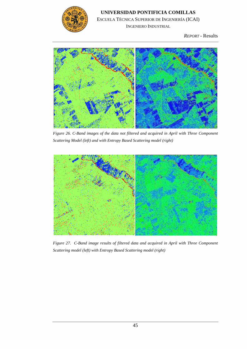
REPORT - Results
45
UNIVERSIDAD PONTIFICIA COMILLAS
ESCUELA TÉCNICA SUPERIOR DE INGENIERÍA (ICAI)
INGENIERO INDUSTRIAL
Figure 26. C-Band images of the data not filtered and acquired in April with Three Component
Scattering Model (left) and with Entropy Based Scattering model (right)
Figure 27. C-Band image results of filtered data and acquired in April with Three Component
Scattering model (left) with Entropy Based Scattering model (right)
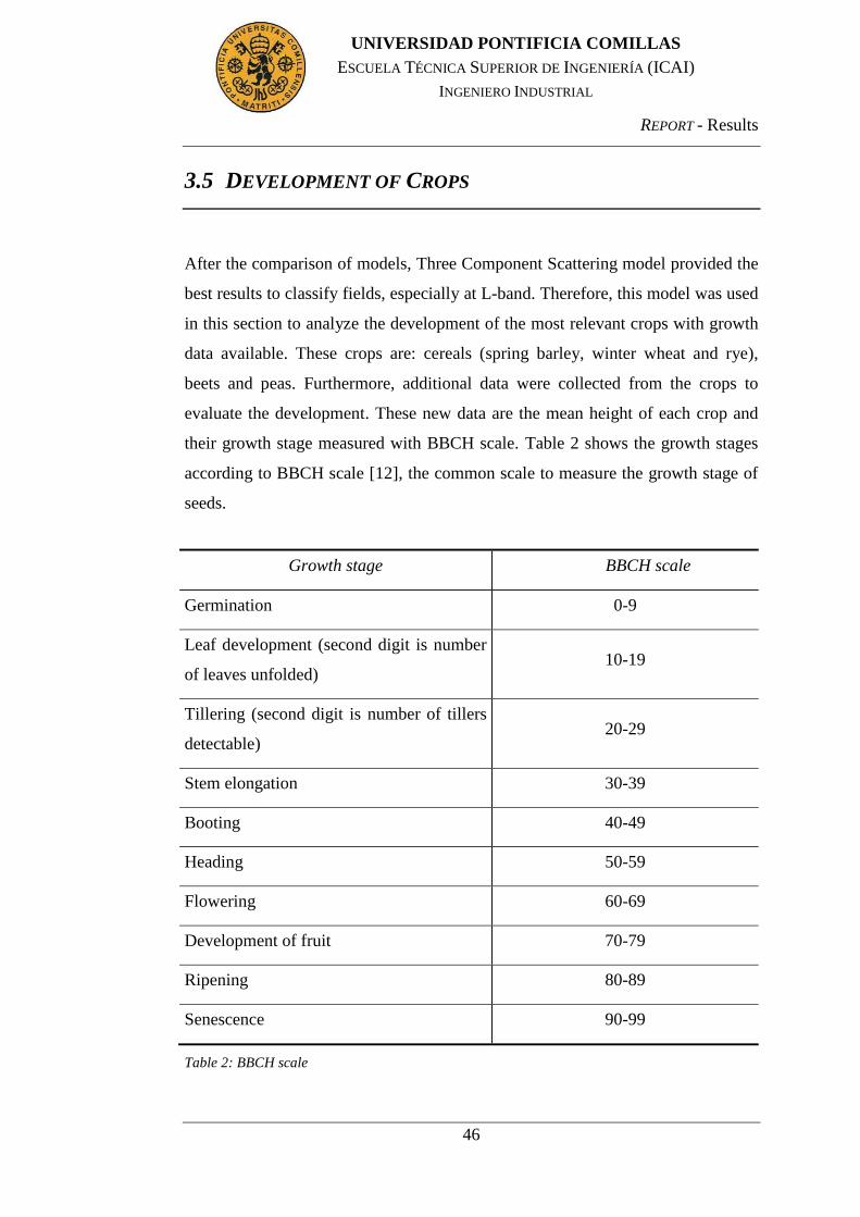
REPORT - Results
46
UNIVERSIDAD PONTIFICIA COMILLAS
ESCUELA TÉCNICA SUPERIOR DE INGENIERÍA (ICAI)
INGENIERO INDUSTRIAL
3.5 DEVELOPMENT OF CROPS
After the comparison of models, Three Component Scattering model provided the
best results to classify fields, especially at L-band. Therefore, this model was used
in this section to analyze the development of the most relevant crops with growth
data available. These crops are: cereals (spring barley, winter wheat and rye),
beets and peas. Furthermore, additional data were collected from the crops to
evaluate the development. These new data are the mean height of each crop and
their growth stage measured with BBCH scale. Table 2 shows the growth stages
according to BBCH scale [12], the common scale to measure the growth stage of
seeds.
Growth stage BBCH scale
Germination 0-9
Leaf development (second digit is number
of leaves unfolded) 10-19
Tillering (second digit is number of tillers
detectable) 20-29
Stem elongation 30-39
Booting 40-49
Heading 50-59
Flowering 60-69
Development of fruit 70-79
Ripening 80-89
Senescence 90-99
Table 2: BBCH scale
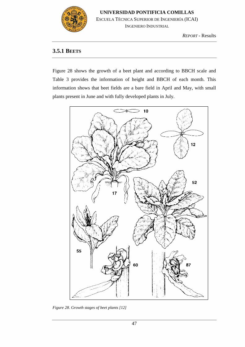
REPORT - Results
47
UNIVERSIDAD PONTIFICIA COMILLAS
ESCUELA TÉCNICA SUPERIOR DE INGENIERÍA (ICAI)
INGENIERO INDUSTRIAL
3.5.1 BEETS
Figure 28 shows the growth of a beet plant and according to BBCH scale and
Table 3 provides the information of height and BBCH of each month. This
information shows that beet fields are a bare field in April and May, with small
plants present in June and with fully developed plants in July.
Figure 28. Growth stages of beet plants [12]

REPORT - Results
48
UNIVERSIDAD PONTIFICIA COMILLAS
ESCUELA TÉCNICA SUPERIOR DE INGENIERÍA (ICAI)
INGENIERO INDUSTRIAL
Table 3: Height and BBCH of beet field from April to July
Figure 29, Figure 30 and Figure 31 illustrate the development of the beet field
from April to July, according to the three scattering powers.
Surface and volume scattering are dominating at L-band. However, a higher
contribution of surface scattering was expected in April and May because of the
bare beet field. This expectation could be not shown as a higher Ps than the other
powers, if the terrain is rough. Therefore, the high and similar powers Pv and Ps
indicate a rough surface of beet crop in April and May.
In addition, for the July acquisition, beet plants are developed with broad leaves,
as it is shown on Table 3. Volume scattering is clearly superior at C-band because
Pv is evidently higher at C-band due to the wavelength of this band, like it occurs
in the other results of this study.
On the other hand, double bounce scattering, shown on Figure 29, is clearly less
predominant due to the shape of beet crops. The first growth stages of beets start
with small and short leaves and it develops to big and large leaves without long
and rigid stems.
Field
April May June July
Height
[cm]
BBCH Height
[cm]
BBCH Height
[cm]
BBCH Height
[cm]
BBCH
30 - - - - - 21 26 35
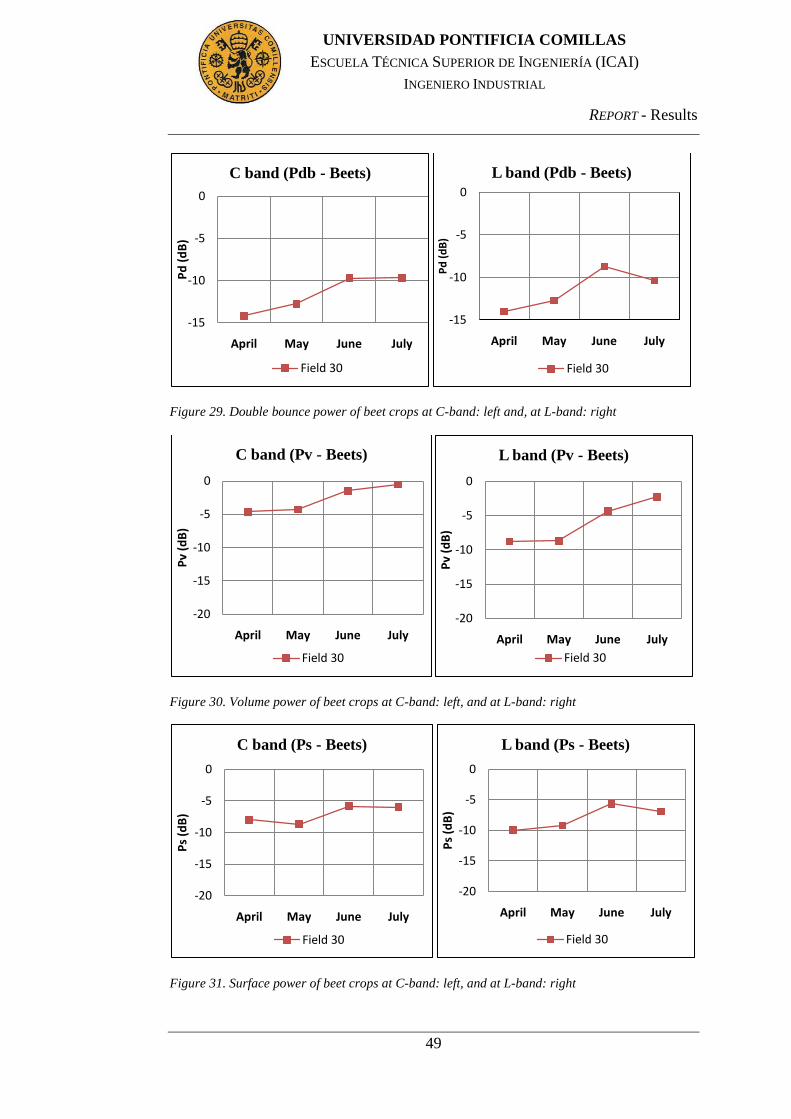
REPORT - Results
49
UNIVERSIDAD PONTIFICIA COMILLAS
ESCUELA TÉCNICA SUPERIOR DE INGENIERÍA (ICAI)
INGENIERO INDUSTRIAL
Figure 29. Double bounce power of beet crops at C-band: left and, at L-band: right
Figure 30. Volume power of beet crops at C-band: left, and at L-band: right
Figure 31. Surface power of beet crops at C-band: left, and at L-band: right
-15
-10
-5
0
April May June July
Pd
(d
B)
C band (Pdb - Beets)
Field 30
-15
-10
-5
0
April May June July
Pd
(d
B)
L band (Pdb - Beets)
Field 30
-20
-15
-10
-5
0
April May June July
Pv
(dB
)
C band (Pv - Beets)
Field 30
-20
-15
-10
-5
0
April May June July
Pv
(dB
)L band (Pv - Beets)
Field 30
-20
-15
-10
-5
0
April May June July
Ps
(dB
)
C band (Ps - Beets)
Field 30
-20
-15
-10
-5
0
April May June July
Ps
(dB
)
L band (Ps - Beets)
Field 30
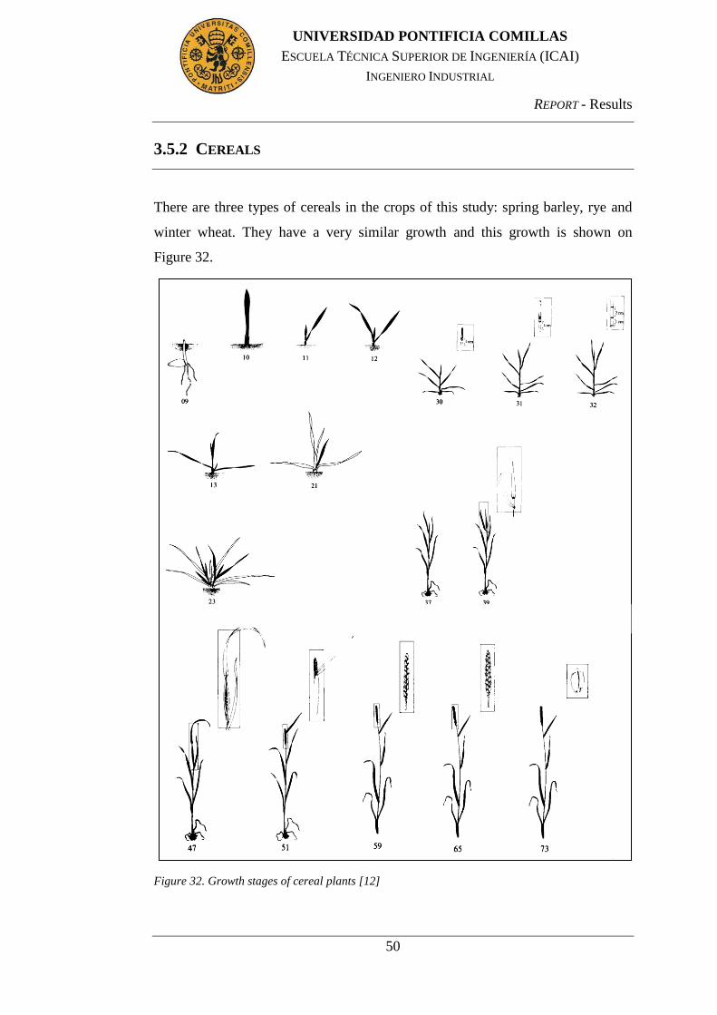
REPORT - Results
50
UNIVERSIDAD PONTIFICIA COMILLAS
ESCUELA TÉCNICA SUPERIOR DE INGENIERÍA (ICAI)
INGENIERO INDUSTRIAL
3.5.2 CEREALS
There are three types of cereals in the crops of this study: spring barley, rye and
winter wheat. They have a very similar growth and this growth is shown on
Figure 32.
Figure 32. Growth stages of cereal plants [12]

REPORT - Results
51
UNIVERSIDAD PONTIFICIA COMILLAS
ESCUELA TÉCNICA SUPERIOR DE INGENIERÍA (ICAI)
INGENIERO INDUSTRIAL
3.5.2.1 Spring barley
Table 4 shows the height and the BBCH of spring barley crops. The height and
BBCH in April is zero because the plant has not started to germinate yet.
Field
April May June July
Height
[cm]
BBCH Height
[cm]
BBCH Height
[cm]
BBCH Height
[cm]
BBCH
6 0 0 14 28 54 49 63 63
13 0 0 15 21 46 41 63 79
36 0 0 11 22-26 62 54 67 86
Table 4. Height and BBCH of spring barley field from April to July
Figure 33 shows the mean of surface power Ps of these crops, Figure 34 shows the
volume scattering and Figure 35 shows the surface scattering at C and L band for
each month.
The scattering from spring barley is dominated by surface at L-band, including the
May acquisitions at this band. The development of these crops seems to be
constant during 4 months, except in the July acquisitions where the three powers
increase about 5 dB.
On the other hand, Figure 34 also shows that the dominating scattering
mechanism at C-band is volume scattering for the all acquisitions and Pv becomes
high, especially in July as at L-band. The dominating volume scattering at C-band
may be due of the short penetration of this band.

REPORT - Results
52
UNIVERSIDAD PONTIFICIA COMILLAS
ESCUELA TÉCNICA SUPERIOR DE INGENIERÍA (ICAI)
INGENIERO INDUSTRIAL
Figure 33. Double bounce power of spring barley crops at C-band: left and, at L-band: right
Figure 34. Volume power of spring barley crops at C-band: left and at L-band: right
Figure 35. Surface power of spring barley crops at C-band: left, and at L-band: right
-20
-15
-10
-5
0
April May June July
Pd
(d
B)
C band (Pdb - Spring barley)
Field 6 Field 13 Field 36
-20
-15
-10
-5
0
April May June July
Pd
(d
B)
L band (Pdb - Spring barley)
Field 6 Field 13 Field 36
-15
-10
-5
0
April May June July
Pv
(dB
)
C band (Pv - Spring barley)
Field 6 Field 13 Field 36
-15
-10
-5
0
April May June July
Pv
(dB
)
L band (Pv - Spring barley)
Field 6 Field 13 Field 36
-15
-10
-5
0
April May June July
Ps
(dB
)
C band (Ps - Spring barley)
Field 6 Field 13 Field 36
-15
-10
-5
0
April May June July
Ps
(dB
)
L band (Ps - Spring barley)
Field 6 Field 13 Field 36

REPORT - Results
53
UNIVERSIDAD PONTIFICIA COMILLAS
ESCUELA TÉCNICA SUPERIOR DE INGENIERÍA (ICAI)
INGENIERO INDUSTRIAL
3.5.2.2 Winter Wheat
The results of winter wheat crop are expected different compared to spring barley
crop. This difference is mainly due to the growth stage of both crops. Table 5
presents the values of height and BBCH of winter wheat crops and the value of
BBCH in April.
Field
April May June July
Height
[cm]
BBCH Height
[cm]
BBCH Height
[cm]
BBCH Height
[cm]
BBCH
3 20 48 37 74 59 71 85
5 14 29 42 39 78 58 90 81
11 30 44 39 73 55 78 85
Table 5: Height and BBCH of winter wheat fields from April to July
The results of the model are shown on Figure 36, Figure 37 and Figure 38 for
double bounce, volume and surface scattering respectively. The height and the
growth stage are similar in the three winter wheat crops for each month and this
can be seen on all Figure 36, Figure 37 and Figure 38, especially in fields 3 and 5.
The scattering of winter wheat is dominated by surface at L-band, except the May
results at L-band which shows dominating double-bounce scattering. On the other
hand, the dominating scattering mechanism at C-band is volume scattering for the
all acquisitions, as it is shown on Figure 36 and Pv becomes high, especially in
July. The scattering presented in field 11 shows a lower volume scattering in the
four months at L-band, this may be due to the rough of the terrain. However, the
dominating scattering mechanism at C-band in field 11 is volume scattering; in
this case the reason is because of the wavelength, shorter at C-band than L-band.
The height of field 5 in July is higher than the other winter wheat crops but no
signs of evidence appeared in the graphics. This may means that BBCH, that
reflects the same growth stage in field 3, 5 and 11, is more significant than height.

REPORT - Results
54
UNIVERSIDAD PONTIFICIA COMILLAS
ESCUELA TÉCNICA SUPERIOR DE INGENIERÍA (ICAI)
INGENIERO INDUSTRIAL
Figure 36. Double bounce power of winter wheat crops at C-band: left, and at L-band: right
Figure 37. Volume power of winter wheat crops at C-band: left, and at L-band: right
Figure 38. Surface power of winter wheat crops at C-band: left, and at L-band: right
-20
-15
-10
-5
0
April May June July
Pd
(d
B)
C band (Pdb - Winter wheat)
Field 3 Field 5 Field 11
-20
-15
-10
-5
0
April May June July
Pd
(d
B)
L band (Pdb -Winter wheat)
Field 3 Field 5 Field 11
-15
-10
-5
0
April May June July
Pv
(dB
)
C band (Pv -Winter wheat)
Field 3 Field 5 Field 11
-15
-10
-5
0
April May June July
Pv
(dB
)L band (Pv -Winter wheat)
Field 3 Field 5 Field 11
-15
-10
-5
0
April May June July
Ps
(dB
)
C band (Ps -Winter wheat)
Field 3 Field 5 Field 11
-15
-10
-5
0
April May June July
Ps
(dB
)
L band (Ps -Winter wheat)
Field 3 Field 5 Field 11

REPORT - Results
55
UNIVERSIDAD PONTIFICIA COMILLAS
ESCUELA TÉCNICA SUPERIOR DE INGENIERÍA (ICAI)
INGENIERO INDUSTRIAL
3.5.2.3 Rye
The results of rye crops are expected similar to winter wheat crops, because they
have very similar features. Table 6 shows the values of height and BBCH of rye
fields.
Table 6: Height and BBCH of rye fields from April to July
The height and the growth stage of the three rye crops are similar for each month,
and the graphics presented on Figure 39, Figure 40 and Figure 41 show the three
scattering mechanisms of each rye crop at both bands. As the case of winter wheat
crops, the May acquisition at L-band shows an increase of double-bounce
scattering. Field 1 shows a more different graphic than the rest of rye fields, with
the lowest values of the powers of all months at L-band. This anomaly may occur
because of edge detection during the filtering. In particular, field 1 has very
irregular crop edges compared to the rest of fields. It is also possible that other
features of crops, not considered in this study, as moisture content can be
responsible of this difference.
Anyway, according to Figure 41, the scattering from rye is dominated by surface
because the power Ps shows the highest values at L-band.
On the other hand, volume scattering is still dominating C-band, but in this case
Pv is higher than in other crops. Besides, volume scattering becomes dominant in
July at L-band due to the development of the vegetation.
Field
April May June July
Height
[cm]
BBCH Height
[cm]
BBCH Height
[cm]
BBCH Height
[cm]
BBCH
1 23-24 61 49 110 60 92 86
8 21 21 51 49 98 65 99 80
12 22 55 63 94 61 88 82
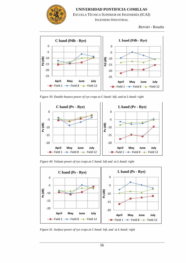
REPORT - Results
56
UNIVERSIDAD PONTIFICIA COMILLAS
ESCUELA TÉCNICA SUPERIOR DE INGENIERÍA (ICAI)
INGENIERO INDUSTRIAL
Figure 39. Double bounce power of rye crops at C-band: left, and at L-band: right
Figure 40. Volume power of rye crops at C-band: left and at L-band: right
Figure 41. Surface power of rye crops at C-band: left, and at L-band: right
-25
-20
-15
-10
-5
0
April May June July
Pd
(d
B)
C band (Pdb - Rye)
Field 1 Field 8 Field 12
-25
-20
-15
-10
-5
0
April May June July
Pd
(d
B)
L band (Pdb - Rye)
Field 1 Field 8 Field 12
-20
-15
-10
-5
0
April May June July
Pv
(dB
)
C band (Pv - Rye)
Field 1 Field 8 Field 12
-20
-15
-10
-5
0
April May June July
Pv
(dB
)L band (Pv - Rye)
Field 1 Field 8 Field 12
-20
-15
-10
-5
0
April May June July
Ps
(dB
)
C band (Ps - Rye)
Field 1 Field 8 Field 12
-20
-15
-10
-5
0
April May June July
Ps
(dB
)
L band (Ps - Rye)
Field 1 Field 8 Field 12
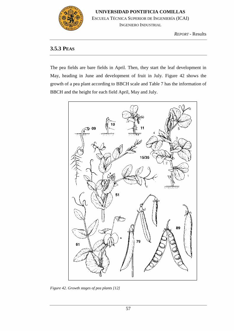
REPORT - Results
57
UNIVERSIDAD PONTIFICIA COMILLAS
ESCUELA TÉCNICA SUPERIOR DE INGENIERÍA (ICAI)
INGENIERO INDUSTRIAL
3.5.3 PEAS
The pea fields are bare fields in April. Then, they start the leaf development in
May, heading in June and development of fruit in July. Figure 42 shows the
growth of a pea plant according to BBCH scale and Table 7 has the information of
BBCH and the height for each field April, May and July.
Figure 42. Growth stages of pea plants [12]

REPORT - Results
58
UNIVERSIDAD PONTIFICIA COMILLAS
ESCUELA TÉCNICA SUPERIOR DE INGENIERÍA (ICAI)
INGENIERO INDUSTRIAL
Table 7: Height and BBCH of pea fields from April to July
Figure 43, Figure 44 and Figure 45 illustrates the mean of each power of each pea
field. The height and the growth stage is almost the same in the three pea crops for
each month and it is reflected in all powers at L-band, except in May where field
18 presents a decrease in each power while the other pea crops show an increase.
Unfortunately, this anomaly cannot explain only with the height and BBCH of the
crop, being necessary other data about the feature of these crops, such as moisture
content.
The powers for pea crops follow the increase of the powers for the beet field but
with a difference of 5 to 10 dB. However, for the July acquisition Pd and Ps
decrease while in pea crops these powers are still increasing.
Moreover, it was expected higher values of Pv in the peas compared to beets.
Because, according to the Table 1 and Table 7, pea crops have developed further
than beets, thus volume scattering would occur in the canopy of pea crops.
Therefore, to distinguish between beets and peas, it would be necessary, another
study of both types of crops, because primarily expectations are not accomplished
and data from only one small field of beets was obtained.
Field
April May June July
Height
[cm]
BBCH Height
[cm]
BBCH Height
[cm]
BBCH Height
[cm]
BBCH
7 0 0 12 14 42 54 69 71
15 0 0 12 14 42 52 69 71
18 0 0 13 14 63 59 52 81
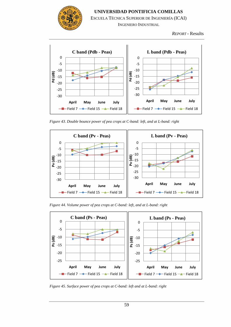
REPORT - Results
59
UNIVERSIDAD PONTIFICIA COMILLAS
ESCUELA TÉCNICA SUPERIOR DE INGENIERÍA (ICAI)
INGENIERO INDUSTRIAL
Figure 43. Double bounce power of pea crops at C-band: left, and at L-band: right
Figure 44. Volume power of pea crops at C-band: left, and at L-band: right
Figure 45. Surface power of pea crops at C-band: left and at L-band: right
-30
-25
-20
-15
-10
-5
0
April May June July
Pd
(d
B)
C band (Pdb - Peas)
Field 7 Field 15 Field 18
-30
-25
-20
-15
-10
-5
0
April May June July
Pd
(d
B)
L band (Pdb - Peas)
Field 7 Field 15 Field 18
-30
-25
-20
-15
-10
-5
0
April May June July
Pv
(dB
)
C band (Pv - Peas)
Field 7 Field 15 Field 18
-30
-25
-20
-15
-10
-5
0
April May June July
Pv
(dB
)
L band (Pv - Peas)
Field 7 Field 15 Field 18
-25
-20
-15
-10
-5
0
April May June July
Ps
(dB
)
C band (Ps - Peas)
Field 7 Field 15 Field 18
-25
-20
-15
-10
-5
0
April May June July
Ps
(dB
)
L band (Ps - Peas)
Field 7 Field 15 Field 18
REPORT - Conclusions
60
UNIVERSIDAD PONTIFICIA COMILLAS
ESCUELA TÉCNICA SUPERIOR DE INGENIERÍA (ICAI)
INGENIERO INDUSTRIAL
Chapter 4 CONCLUSIONS
The objectives of this project were fully accomplished, showing that Three
Component Scattering model and Entropy Based Scattering model are two
decomposition models that can be implemented in MATLAB, and they produce
useful results to classify some agricultural areas and monitor their development.
Nevertheless, the presence of speckle and errors in the SAR data used may
produce the misunderstanding of some fields. For this reason, it was necessary to
analyze SAR data before their interpretation and also to apply a filter before the
implementation of the models. Besides, additional data about the crops, apart of
BBCH and height, would be interesting to analyze with the results of these
models.
4.1 IMPLEMENTATION
During the implementation, data analysis shows that polarimetric SAR data do not
totally fit the Three Component Scattering model. However, that does not have
great influence on the accuracy of the obtained results. As the number of
deviations of element amplitudes is not larger than 200 in this particular
image the error is about 0.02%, which indicates that the SAR data accuracy is
very high.
Moreover, Entropy Based Scattering model detected an error in one of the SAR
images. The error appeared in the calculation of entropy and alpha when some
pixels had a value outside the limits (H<0 and α>90º). However, Three-
Component Scattering model could not discover this error during its
implementation or its result.
REPORT - Conclusions
61
UNIVERSIDAD PONTIFICIA COMILLAS
ESCUELA TÉCNICA SUPERIOR DE INGENIERÍA (ICAI)
INGENIERO INDUSTRIAL
4.2 RESULTS
Three Component Scattering model was a useful tool to analyze the development
of crops. The analysis of winter crops, such as winter wheat, rye and grass, shows
a dominant double bounce scattering in May due to the shape of the winter crop
and the growth state at that date, especially at L-band. On the other hand, spring
crops present some differences in scattering among them. The reason of these
differences is that they are different type of crops, with different shape and growth
stages. However, since only data from one beet crop were available, it is possible
that the comparison were not enough accurate. Furthermore, volume scattering
was dominant at C-band in all of the fields because the penetration of this band is
very limited compared to L-band.
The application of a speckle filter improved the image markedly. Speckle was
sufficiently reduced and edges of areas were not blurred that indicates that the
chosen size of the moving window was appropriate for edge directions detection
and the estimation of the value of noise variance was likely accurate.
After the comparison of both models, the results of the SAR images were more
satisfactory in Three Component Scattering model at L-band. However, better
results were found with the other model, Entropy Based Scattering model, at C-
band.
REPORT - Future Work
62
UNIVERSIDAD PONTIFICIA COMILLAS
ESCUELA TÉCNICA SUPERIOR DE INGENIERÍA (ICAI)
INGENIERO INDUSTRIAL
Chapter 5 FUTURE WORK
It is possible to apply statistical classifiers to distinguish in more detail different
types of crops. A good recommendation is to use a classifier called “Wishart
classifier” [13]. It needs some iterations to see significant results and can be used
in both models. However, with Entropy Based Scattering model create wrong
final results because a pixel can change the zone during the iterations and thus, a
pixel can end at a wrong scattering mechanism. This problem does not occur with
Three Component Scattering model because it already has a previous
classification in the three common scattering mechanisms.
In addition, some studies indicate that Entropy Based Scattering model needs
another variable to classify with precision. Thus, this model may be further
improved by explicitly including the anisotropy information during the
segmentation procedure with the Wishart classifier. The anisotropy indicates the
relative importance of secondary mechanisms obtained from the expansion of a
coherency matrix. This polarimetric indicator is particularly useful to discriminate
scattering mechanisms with different eigenvalue distributions but with similar
intermediate entropy values.
Moreover, although a speckle filter was successfully implemented, it is possible to
improve it, reducing the speckle but keeping as much information as possible. In
this way, the edge detection may have more type of windows, including one
without edges. Besides, different sizes of the window may adjust better to edges
of some fields, thus windows with different sizes may be implemented.

USER GUIDE
63
UNIVERSIDAD PONTIFICIA COMILLAS
ESCUELA TÉCNICA SUPERIOR DE INGENIERÍA (ICAI)
INGENIERO INDUSTRIAL
BIBLIOGRAPHY
[1] J. A. Richards, Remote sensing with Radar Imaging, Springer. Verlag, Berlin,
Heidelberg, 2009.
[2] J. J. van Zyl, and F. T. Ulaby, Scattering Matrix Representation for Simple
Targets, in F. T. Ulaby and C. Elachi (editors), Radar Polarimetry for
Geoscience Applications, Norwood, Artech House, Inc. 1990.
[3] A. Freeman, S. L. Durden, A Three-component Scattering Model for
Polarimetric SAR Data. May, 1998.
[4] S. R. Cloude, E. Pottier, An Entropy Based Classification scheme for Land
Applications for Polarimetric SAR. January, 1997.
[5] J. Lee, M. R. Grunes, T. L. Ainsworth, L. Du, D. L. Schuler, S. R. Cloude,
Unsupervised Classification Using Polarimetric Decomposition and the Complex
Wishart Classifier. September, 1999.
[6] A. C. Frery, A. Correia, C. D. Rennó, C. C. Freitas, J. Jacobo-Berlles, K. L. P.
Vasconcellos, M. Mejail, S. J. S. Sant’ann, Models for Synthetic Aperture Radar
Image Analysis. Brazil, Argentina. 2009.
[7] ESA Earthnet Online. Temporal Averaging [Online]
http://earth.esa.int/applications/data_util/SARDOCS/spaceborne/Radar_Courses/
Radar_Course_III/temporal_averaging.htm consulted on 25th January 2011.
[8] J. Lee, M. R. Grunes, G. de Grandi. Polarimetric SAR Speckle Filtering and Its
Implication for Classification. September, 1999.
[9] F. T. Ulaby, R. K. Moore, and A. K. Fung, Microwave Remote Sensing: Active
and Passive, vol. 3. Dedham, MA: Artech, 1986.
[10] MATLAB® 7. Documentation - Data Analysis. MathWorks. [Online]
http://www.mathworks.com/help/techdoc/data_analysis/ug_intropage.html
consulted on 25th January.

USER GUIDE
64
UNIVERSIDAD PONTIFICIA COMILLAS
ESCUELA TÉCNICA SUPERIOR DE INGENIERÍA (ICAI)
INGENIERO INDUSTRIAL
[11] MATLAB® 7. Documentation - Mathematics. MathWorks. [Online]
http://www.mathworks.com/help/techdoc/math/bqqz59g.html consulted on 25th
January.
[12] U. Meier, Growth stages of mono-and dicotyledonous plants. BBCH Monograph,
2 ed. Federal Biological Research Centre for Agriculture and Forestry, 2001.
[13] J. Lee, M. R. Grunes, R. Kwok, Classification of multi-look polarimetric SAR
imagery based on complex Wishart distribution. November, 1994.
[14] J. Lee, M. R. Grunes, E. Pottier, L. Ferro-Famil, Unsupervised Terrain
Classification Preserving Polarimetric Scattering Characteristics. April, 2004.

USER GUIDE
65
UNIVERSIDAD PONTIFICIA COMILLAS
ESCUELA TÉCNICA SUPERIOR DE INGENIERÍA (ICAI)
INGENIERO INDUSTRIAL
Part II USER GUIDE

USER GUIDE - MATLAB Programming
66
UNIVERSIDAD PONTIFICIA COMILLAS
ESCUELA TÉCNICA SUPERIOR DE INGENIERÍA (ICAI)
INGENIERO INDUSTRIAL
Chapter 1 MATLAB PROGRAMMING
MATLAB allows sequences of instructions to be stored in so-called M-files.
An M-file has the following structure:
• The function definition line
• The H1 line
• Help text
• The function body
• Comments
The function definition line looks like:
function [outputs] = function_name(inputs)
For example, a function to split a colour image into its R, G, and B components
would look like:
function [R, G, B] = split_colour_planes(src)
This would be called at the command prompt as:
>> [r, g, b] = split_colour_planes(a_colour_image);
There are restrictions on the form of function names: they must begin with a
letter, can’t contain any spaces and only the first 63 characters are significant. If
the function has no output, the square brackets and equal sign are omitted. If the
function has a single output, the square brackets may be omitted.

USER GUIDE - MATLAB Programming
67
UNIVERSIDAD PONTIFICIA COMILLAS
ESCUELA TÉCNICA SUPERIOR DE INGENIERÍA (ICAI)
INGENIERO INDUSTRIAL
The H1 line follows the definition line with no blank lines of leading spaces. It is
a comment that Matlab returns first when help is invoked, and is searched for
keywords when look for keyword is used. The format of the H1 line is
% function_name <text description>
The help text must follow with no blank lines. The lines up to the next blank line
are also printed by help. Each line of help text must start with a % symbol.
Other lines stating with the % symbol are treated simply as comments for the
programmer.
The function body can contain any instruction that would be valid at the command
line.
Matlab provides the usual programming constructs, but (naturally) the syntax is
different to other languages.
Conditional execution:
if expression
statement(s)
end
OR
if expression1
statement1
elseif expression2
statement2
else
statement3

USER GUIDE - MATLAB Programming
68
UNIVERSIDAD PONTIFICIA COMILLAS
ESCUELA TÉCNICA SUPERIOR DE INGENIERÍA (ICAI)
INGENIERO INDUSTRIAL
end
For loop:
for index = start:increment:end
statements
end

PROGRAMMING CODE
69
UNIVERSIDAD PONTIFICIA COMILLAS
ESCUELA TÉCNICA SUPERIOR DE INGENIERÍA (ICAI)
INGENIERO INDUSTRIAL
Part III PROGRAMMING
CODE

PROGRAMMING CODE - Three Component Scattering model
70
UNIVERSIDAD PONTIFICIA COMILLAS
ESCUELA TÉCNICA SUPERIOR DE INGENIERÍA (ICAI)
INGENIERO INDUSTRIAL
Chapter 1 THREE COMPONENT SCATTERING
MODEL
%%%%%%%%%%%%%%%%%%%%%%%%%%%%%%%%%%%%%%%%%%%%%%%%%%%%%%%%%%%%%%%%%%%%%%%%%
% Unsupervised Classification of Polarimetric SAR Data %
%%%%%%%%%%%%%%%%%%%%%%%%%%%%%%%%%%%%%%%%%%%%%%%%%%%%%%%%%%%%%%%%%%%%%%%%%
%%%%%%%%%%%%%%%%%%%%%% 3 COMPONENT SCATTERING MODEL %%%%%%%%%%%%%%%%%%%%%
%%%%%%%%% Open SAR data and Calculation of Covariance matrix %%%%%%%%%%%%
clear all
clc
file_hhhh=fopen('hhhh.dat','r','b');
hhhh=fread(file_hhhh,[1,inf],'float32');
fclose(file_hhhh);
file_hhhv=fopen('hhhv.dat','r','b');
hhhv0=fread(file_hhhv,[2,inf],'float32');
hhhv=hhhv0(1,:)+j*hhhv0(2,:);
fclose(file_hhhv);
file_hvhv=fopen('hvhv.dat','r','b');
hvhv=fread(file_hvhv,[1,inf],'float32');
fclose(file_hvhv);
file_hhvv = fopen('hhvv.dat','r','b');
hhvv0=fread(file_hhvv,[2,inf],'float32');
hhvv=hhvv0(1,:)+j*hhvv0(2,:);
fclose(file_hhvv);
file_hvvv = fopen('hvvv.dat','r','b');
hvvv0=fread(file_hvvv,[2,inf],'float32');
hvvv=hvvv0(1,:)+j*hvvv0(2,:);
fclose(file_hvvv);
file_vvvv = fopen('vvvv.dat','r','b');

PROGRAMMING CODE - Three Component Scattering model
71
UNIVERSIDAD PONTIFICIA COMILLAS
ESCUELA TÉCNICA SUPERIOR DE INGENIERÍA (ICAI)
INGENIERO INDUSTRIAL
vvvv=fread(file_vvvv,[1,inf],'float32');
fclose(file_vvvv);
l=length(hhhh);
CM=zeros(3,3,l);
CM(1,1,:)=hhhh;
CM(1,2,:)=sqrt(2)*hhhv;
CM(1,3,:)=hhvv;
CM(2,1,:)=sqrt(2)*conj(hhhv);
CM(2,2,:)=2*hvhv;
CM(2,3,:)=sqrt(2)*hvvv;
CM(3,1,:)=conj(hhhv);
CM(3,2,:)=sqrt(2)*(hvvv);
CM(3,3,:)
else
fd=r(3);
end
fs=b-fd;
alfa=(k-fs)/fd+(m/fd)*1i;
fv=3*CovMat(2,2);
Ps=fs*(1+beta^2);
Pd=fd*(1+alfa^2);
Pv=8*fv/3;
end
% These powers are the real value but it is necessary to convert the
scala into logarithm scala %
% Power_matrix(ii,1)=Pd; %
% Power_matrix(ii,2)=Pv; %
% Power_matrix(ii,3)=Ps; %
Power_matrix(ii,1)=10*log10(abs(Pd));
Power_matrix(ii,2)=10*log10(abs(Pv));
Power_matrix(ii,3)=10*log10(abs(Ps));
end
%%%%%%%%%%%%%%%%%%%%%%%%%%%%%%%%%%%%%%%%%%%%%%%%%%%%%%%%%%%%%%%%%%%%%%%%%

PROGRAMMING CODE - Three Component Scattering model
72
UNIVERSIDAD PONTIFICIA COMILLAS
ESCUELA TÉCNICA SUPERIOR DE INGENIERÍA (ICAI)
INGENIERO INDUSTRIAL
%%%%%%%%%%%%%% HISTOGRAMS (to see the data distribution) %%%%%%%%%%%%%%%%
x = 50;
y = Power_matrix(:,1);
hist(y,x); title('Double Bounce');
figure
hold on
y = Power_matrix(:,2); title('Volume');
hist(y,x)
figure
hold on
y = Power_matrix(:,3); title('Surface');
hist(y,x)
%%%%%%%%%%%%%%%%%%%%%%%%%%%%%%%%%%%%%%%%%%%%%%%%%%%%%%%%%%%%%%%%%%%%%%%%%
%%%%%%%%%%%%%%%%%%%%%%%% IMAGE REPRESENTATION %%%%%%%%%%%%%%%%%%%%%%%%%%%
nstd = 2;
image1 = Power_matrix(:,1)-repmat(mean(Power_matrix(:,1)),1024*1024, 1);
image2 = Power_matrix(:,2)-repmat(mean(Power_matrix(:,2)),1024*1024, 1);
image3 = Power_matrix(:,3)-repmat(mean(Power_matrix(:,3)),1024*1024, 1);
stdvar1 = std(image1);
stdvar2 = std(image2);
stdvar3 = std(image3);
image1 = reshape(image1, 1024, 1024)';
image2 = reshape(image2, 1024, 1024)';
image3 = reshape(image3, 1024, 1024)';
r = image1/(2*nstd*stdvar1)+0.5;
g = image2/(2*nstd*stdvar2)+0.5;
b = image3/(5*nstd*stdvar3)+0.6;
figure
imshow(cat(3,r,g,b))
%%%%%%%%%%%%%%%%%%%%%%%%%%%%%%%%%%%%%%%%%%%%%%%%%%%%%%%%%%%%%%%%%%%%%%%%%

PROGRAMMING CODE - Three Component Scattering model
73
UNIVERSIDAD PONTIFICIA COMILLAS
ESCUELA TÉCNICA SUPERIOR DE INGENIERÍA (ICAI)
INGENIERO INDUSTRIAL
%%%%%%%%%%%%% Calculation of MEAN POWERS OF EACH FIELD %%%%%%%%%%%%%%%%%%
mean_P=zeros(26,2);
%%%%%%%%%%%%%%%%%%%%%%% Field 4 (grass) %%%%%%%%%%%%%%%%%%%%%%%%%%%%%%%%%
pixels_square_grass= zeros(70,70);
y_pixels=260;
image_Pdb = reshape(Power_matrix(:,1), 1024, 1024)';
image_Pv = reshape(Power_matrix(:,2), 1024, 1024)';
image_Ps = reshape(Power_matrix(:,3), 1024, 1024)';
for ysquare_pixels=1:70 % 70 is the number of pixels in y direction %
x_pixels=150;
for xsquare_pixels=1:70 % 70 is the number of pixels in x direction %
pixels_square_Pdb_1(xsquare_pixels,ysquare_pixels) =
image_Pdb(x_pixels,y_pixels);
pixels_square_Pv_1(xsquare_pixels,ysquare_pixels) =
image_Pv(x_pixels,y_pixels);
pixels_square_Ps_1(xsquare_pixels,ysquare_pixels) =
image_Ps(x_pixels,y_pixels);
x_pixels=x_pixels+1;
end
y_pixels=y_pixels+1;
end
pixels_notsquare_Pdb=reshape(pixels_square_Pdb_1,1,4900);
pixels_notsquare_Pv=reshape(pixels_square_Pv_1,1,4900);
pixels_notsquare_Ps=reshape(pixels_square_Ps_1,1,4900);
mean_P(1,1)=mean(pixels_notsquare_Pdb);
mean_P(1,2)=mean(pixels_notsquare_Pv);
mean_P(1,3)=mean(pixels_notsquare_Ps);
%%%%%%%%%%%%%%%%%%%%%%%%%%%%%%%%%%%%%%%%%%%%%%%%%%%%%%%%%%%%%%%%%%%%%%%%%
%%%%%%%%%%%%%%%%%%%%%%%% Field 30 (beets)%%%%%%%%%%%%%%%%%%%%%%%%%%%%%%%%
pixels_square_beet= zeros(20,15);
y_pixels=70;
image_Pdb = reshape(Power_matrix(:,1), 1024, 1024)';
image_Pv = reshape(Power_matrix(:,2), 1024, 1024)';
image_Ps = reshape(Power_matrix(:,3), 1024, 1024)';
for ysquare_pixels=1:15 % 15 is the number of pixels in y direction %
x_pixels=260;
for xsquare_pixels=1:15 % 15 is the number of pixels in x direction %
pixels_square_Pdb_2(xsquare_pixels,ysquare_pixels) =
image_Pdb(x_pixels,y_pixels);
pixels_square_Pv_2(xsquare_pixels,ysquare_pixels) =

PROGRAMMING CODE - Three Component Scattering model
74
UNIVERSIDAD PONTIFICIA COMILLAS
ESCUELA TÉCNICA SUPERIOR DE INGENIERÍA (ICAI)
INGENIERO INDUSTRIAL
image_Pv(x_pixels,y_pixels);
pixels_square_Ps_2(xsquare_pixels,ysquare_pixels) =
image_Ps(x_pixels,y_pixels);
x_pixels=x_pixels+1;
end
y_pixels=y_pixels+1;
end
pixels_notsquare_Pdb=reshape(pixels_square_Pdb_2,1,4900);
pixels_notsquare_Pv=reshape(pixels_square_Pv_2,1,4900);
pixels_notsquare_Ps=reshape(pixels_square_Ps_2,1,4900);
mean_P(2,1)=mean(pixels_notsquare_Pdb);
mean_P(2,2)=mean(pixels_notsquare_Pv);
mean_P(2,3)=mean(pixels_notsquare_Ps);
%%%%%%%%%%%%%%%%%%%%%%%%%%%%%%%%%%%%%%%%%%%%%%%%%%%%%%%%%%%%%%%%%%%%%%%%%
%%%%%%%%%%%%%%%%%%%% Field 5 (winter wheat) %%%%%%%%%%%%%%%%%%%%%%%%%%%%%
y_pixels=340;
image_Pdb = reshape(Power_matrix(:,1), 1024, 1024)';
image_Pv = reshape(Power_matrix(:,2), 1024, 1024)';
image_Ps = reshape(Power_matrix(:,3), 1024, 1024)';
for ysquare_pixels=1:70 % 70 is the number of pixels in y direction %
x_pixels=220;
for xsquare_pixels=1:70 % 70 is the number of pixels in x direction %
pixels_square_Pdb_3(xsquare_pixels,ysquare_pixels) =
image_Pdb(x_pixels,y_pixels);
pixels_square_Pv_3(xsquare_pixels,ysquare_pixels) =
image_Pv(x_pixels,y_pixels);
pixels_square_Ps_3(xsquare_pixels,ysquare_pixels) =
image_Ps(x_pixels,y_pixels);
x_pixels=x_pixels+1;
end
y_pixels=y_pixels+1;
end
pixels_notsquare_Pdb=reshape(pixels_square_Pdb_3,1,4900);
pixels_notsquare_Pv=reshape(pixels_square_Pv_3,1,4900);
pixels_notsquare_Ps=reshape(pixels_square_Ps_3,1,4900);
mean_P(3,1)=mean(pixels_notsquare_Pdb);
mean_P(3,2)=mean(pixels_notsquare_Pv);
mean_P(3,3)=mean(pixels_notsquare_Ps);
%%%%%%%%%%%%%%%%%%%%%%%%%%%%%%%%%%%%%%%%%%%%%%%%%%%%%%%%%%%%%%%%%%%%%%%%%
%%%%%%%%%%%%%%%%%%%%%% Field 11 (winter wheat)%%%%%%%%%%%%%%%%%%%%%%%%%%%

PROGRAMMING CODE - Three Component Scattering model
75
UNIVERSIDAD PONTIFICIA COMILLAS
ESCUELA TÉCNICA SUPERIOR DE INGENIERÍA (ICAI)
INGENIERO INDUSTRIAL
y_pixels=540;
image_Pdb = reshape(Power_matrix(:,1), 1024, 1024)';
image_Pv = reshape(Power_matrix(:,2), 1024, 1024)';
image_Ps = reshape(Power_matrix(:,3), 1024, 1024)';
for ysquare_pixels=1:60 % 60 is the number of pixels in y direction %
x_pixels=420;
for xsquare_pixels=1:60 % 60 is the number of pixels in x direction %
pixels_square_Pdb_4(xsquare_pixels,ysquare_pixels) =
image_Pdb(x_pixels,y_pixels);
pixels_square_Pv_4(xsquare_pixels,ysquare_pixels) =
image_Pv(x_pixels,y_pixels);
pixels_square_Ps_4(xsquare_pixels,ysquare_pixels) =
image_Ps(x_pixels,y_pixels);
x_pixels=x_pixels+1;
end
y_pixels=y_pixels+1;
end
pixels_notsquare_Pdb=reshape(pixels_square_Pdb_2,1,3600);
pixels_notsquare_Pv=reshape(pixels_square_Pv_2,1,3600);
pixels_notsquare_Ps=reshape(pixels_square_Ps_2,1,3600);
mean_P(2,1)=mean(pixels_notsquare_Pdb);
mean_P(2,2)=mean(pixels_notsquare_Pv);
mean_P(2,3)=mean(pixels_notsquare_Ps);
%%%%%%%%%%%%%%%%%%%%%%%%%%%%%%%%%%%%%%%%%%%%%%%%%%%%%%%%%%%%%%%%%%%%%%%%%
%%%%%%%%%%%%%%%%%%%%%%% Field 20 (winter wheat) %%%%%%%%%%%%%%%%%%%%%%%%%
y_pixels=585;
image_Pdb = reshape(Power_matrix(:,1), 1024, 1024)';
image_Pv = reshape(Power_matrix(:,2), 1024, 1024)';
image_Ps = reshape(Power_matrix(:,3), 1024, 1024)';
for ysquare_pixels=1:40 % 40 is the number of pixels in y direction %
x_pixels=785;
for xsquare_pixels=1:40 % 40 is the number of pixels in x direction %
pixels_square_Pdb_3(xsquare_pixels,ysquare_pixels) =
image_Pdb(x_pixels,y_pixels);
pixels_square_Pv_3(xsquare_pixels,ysquare_pixels) =
image_Pv(x_pixels,y_pixels);
pixels_square_Ps_3(xsquare_pixels,ysquare_pixels) =
image_Ps(x_pixels,y_pixels);
x_pixels=x_pixels+1;
end
y_pixels=y_pixels+1;

PROGRAMMING CODE - Three Component Scattering model
76
UNIVERSIDAD PONTIFICIA COMILLAS
ESCUELA TÉCNICA SUPERIOR DE INGENIERÍA (ICAI)
INGENIERO INDUSTRIAL
end
pixels_notsquare_Pdb=reshape(pixels_square_Pdb_3,1,1600);
pixels_notsquare_Pv=reshape(pixels_square_Pv_3,1,1600);
pixels_notsquare_Ps=reshape(pixels_square_Ps_3,1,1600);
mean_P(3,1)=mean(pixels_notsquare_Pdb);
mean_P(3,2)=mean(pixels_notsquare_Pv);
mean_P(3,3)=mean(pixels_notsquare_Ps);
%%%%%%%%%%%%%%%%%%%%%%%%%%%%%%%%%%%%%%%%%%%%%%%%%%%%%%%%%%%%%%%%%%%%%%%%%
%%%%%%%%%%%%%%%%%%%%%%% Field 27 (winter wheat) %%%%%%%%%%%%%%%%%%%%%%%%%
y_pixels=970;
image_Pdb = reshape(Power_matrix(:,1), 1024, 1024)';
image_Pv = reshape(Power_matrix(:,2), 1024, 1024)';
image_Ps = reshape(Power_matrix(:,3), 1024, 1024)';
for ysquare_pixels=1:40 % 40 is the number of pixels in y direction %
x_pixels=690;
for xsquare_pixels=1:40 % 40 is the number of pixels in x direction %
pixels_square_Pdb_4(xsquare_pixels,ysquare_pixels) =
image_Pdb(x_pixels,y_pixels);
pixels_square_Pv_4(xsquare_pixels,ysquare_pixels) =
image_Pv(x_pixels,y_pixels);
pixels_square_Ps_4(xsquare_pixels,ysquare_pixels) =
image_Ps(x_pixels,y_pixels);
x_pixels=x_pixels+1;
end
y_pixels=y_pixels+1;
end
pixels_notsquare_Pdb=reshape(pixels_square_Pdb_4,1,1600);
pixels_notsquare_Pv=reshape(pixels_square_Pv_4,1,1600);
pixels_notsquare_Ps=reshape(pixels_square_Ps_4,1,1600);
mean_P(4,1)=mean(pixels_notsquare_Pdb);
mean_P(4,2)=mean(pixels_notsquare_Pv);
mean_P(4,3)=mean(pixels_notsquare_Ps);
%%%%%%%%%%%%%%%%%%%%%%%%%%%%%%%%%%%%%%%%%%%%%%%%%%%%%%%%%%%%%%%%%%%%%%%%%
%%%%%%%%%%%%%%%%%%%%% Field 33 (winter wheat)%%%%%%%%%%%%%%%%%%%%%%%%%%%%
y_pixels=75;
image_Pdb = reshape(Power_matrix(:,1), 1024, 1024)';
image_Pv = reshape(Power_matrix(:,2), 1024, 1024)';
image_Ps = reshape(Power_matrix(:,3), 1024, 1024)';
for ysquare_pixels=1:30 % 30 is the number of pixels in y direction %
x_pixels=90;

PROGRAMMING CODE - Three Component Scattering model
77
UNIVERSIDAD PONTIFICIA COMILLAS
ESCUELA TÉCNICA SUPERIOR DE INGENIERÍA (ICAI)
INGENIERO INDUSTRIAL
for xsquare_pixels=1:30 % 30 is the number of pixels in x direction %
pixels_square_Pdb_5(xsquare_pixels,ysquare_pixels) =
image_Pdb(x_pixels,y_pixels);
pixels_square_Pv_5(xsquare_pixels,ysquare_pixels) =
image_Pv(x_pixels,y_pixels);
pixels_square_Ps_5(xsquare_pixels,ysquare_pixels) =
image_Ps(x_pixels,y_pixels);
x_pixels=x_pixels+1;
end
y_pixels=y_pixels+1;
end
pixels_notsquare_Pdb=reshape(pixels_square_Pdb_5,1,900);
pixels_notsquare_Pv=reshape(pixels_square_Pv_5,1,900);
pixels_notsquare_Ps=reshape(pixels_square_Ps_5,1,900);
mean_P(5,1)=mean(pixels_notsquare_Pdb);
mean_P(5,2)=mean(pixels_notsquare_Pv);
mean_P(5,3)=mean(pixels_notsquare_Ps);
%%%%%%%%%%%%%%%%%%%%%%%%%%%%%%%%%%%%%%%%%%%%%%%%%%%%%%%%%%%%%%%%%%%%%%%%%
%%%%%%%%%%%%%%%%%%%%%%%% Field 6 (spring barley) %%%%%%%%%%%%%%%%%%%%%%%%
y_pixels=450;
image_Pdb = reshape(Power_matrix(:,1), 1024, 1024)';
image_Pv = reshape(Power_matrix(:,2), 1024, 1024)';
image_Ps = reshape(Power_matrix(:,3), 1024, 1024)';
for ysquare_pixels=1:50 % 50 is the number of pixels in y direction %
x_pixels=230;
for xsquare_pixels=1:50 % 50 is the number of pixels in x direction %
pixels_square_Pdb_6(xsquare_pixels,ysquare_pixels) =
image_Pdb(x_pixels,y_pixels);
pixels_square_Pv_6(xsquare_pixels,ysquare_pixels) =
image_Pv(x_pixels,y_pixels);
pixels_square_Ps_6(xsquare_pixels,ysquare_pixels) =
image_Ps(x_pixels,y_pixels);
x_pixels=x_pixels+1;
end
y_pixels=y_pixels+1;
end
pixels_notsquare_Pdb=reshape(pixels_square_Pdb_6,1,4900);
pixels_notsquare_Pv=reshape(pixels_square_Pv_6,1,4900);
pixels_notsquare_Ps=reshape(pixels_square_Ps_6,1,4900);
mean_P(6,1)=mean(pixels_notsquare_Pdb);

PROGRAMMING CODE - Three Component Scattering model
78
UNIVERSIDAD PONTIFICIA COMILLAS
ESCUELA TÉCNICA SUPERIOR DE INGENIERÍA (ICAI)
INGENIERO INDUSTRIAL
mean_P(6,2)=mean(pixels_notsquare_Pv);
mean_P(6,3)=mean(pixels_notsquare_Ps);
%%%%%%%%%%%%%%%%%%%%%%%%%%%%%%%%%%%%%%%%%%%%%%%%%%%%%%%%%%%%%%%%%%%%%%%%%
%%%%%%%%%%%%%%%%%%%% Field 13 (spring barley) %%%%%%%%%%%%%%%%%%%%%%%%%%%
y_pixels=728;
image_Pdb = reshape(Power_matrix(:,1), 1024, 1024)';
image_Pv = reshape(Power_matrix(:,2), 1024, 1024)';
image_Ps = reshape(Power_matrix(:,3), 1024, 1024)';
for ysquare_pixels=1:30 % 30 is the number of pixels in y direction %
x_pixels=428;
for xsquare_pixels=1:30 % 30 is the number of pixels in x direction %
pixels_square_Pdb_7(xsquare_pixels,ysquare_pixels) =
image_Pdb(x_pixels,y_pixels);
pixels_square_Pv_7(xsquare_pixels,ysquare_pixels) =
image_Pv(x_pixels,y_pixels);
pixels_square_Ps_7(xsquare_pixels,ysquare_pixels) =
image_Ps(x_pixels,y_pixels);
x_pixels=x_pixels+1;
end
y_pixels=y_pixels+1;
end
pixels_notsquare_Pdb=reshape(pixels_square_Pdb_7,1,4900);
pixels_notsquare_Pv=reshape(pixels_square_Pv_7,1,4900);
pixels_notsquare_Ps=reshape(pixels_square_Ps_7,1,4900);
mean_P(7,1)=mean(pixels_notsquare_Pdb);
mean_P(7,2)=mean(pixels_notsquare_Pv);
mean_P(7,3)=mean(pixels_notsquare_Ps);
%%%%%%%%%%%%%%%%%%%%%%%%%%%%%%%%%%%%%%%%%%%%%%%%%%%%%%%%%%%%%%%%%%%%%%%%%
%%%%%%%%%%%%%%%%%%%% Field 14 (spring barley) %%%%%%%%%%%%%%%%%%%%%%%%%%
y_pixels=700;
image_Pdb = reshape(Power_matrix(:,1), 1024, 1024)';
image_Pv = reshape(Power_matrix(:,2), 1024, 1024)';
image_Ps = reshape(Power_matrix(:,3), 1024, 1024)';
for ysquare_pixels=1:10 % 10 is the number of pixels in y direction %
x_pixels=490;
for xsquare_pixels=1:10 % 10 is the number of pixels in x direction %
pixels_square_Pdb_8(xsquare_pixels,ysquare_pixels) =
image_Pdb(x_pixels,y_pixels);
pixels_square_Pv_8(xsquare_pixels,ysquare_pixels) =
image_Pv(x_pixels,y_pixels);

PROGRAMMING CODE - Three Component Scattering model
79
UNIVERSIDAD PONTIFICIA COMILLAS
ESCUELA TÉCNICA SUPERIOR DE INGENIERÍA (ICAI)
INGENIERO INDUSTRIAL
pixels_square_Ps_8(xsquare_pixels,ysquare_pixels) =
image_Ps(x_pixels,y_pixels);
x_pixels=x_pixels+1;
end
y_pixels=y_pixels+1;
end
pixels_notsquare_Pdb=reshape(pixels_square_Pdb_8,1,100);
pixels_notsquare_Pv=reshape(pixels_square_Pv_8,1,100);
pixels_notsquare_Ps=reshape(pixels_square_Ps_8,1,100);
mean_P(8,1)=mean(pixels_notsquare_Pdb);
mean_P(8,2)=mean(pixels_notsquare_Pv);
mean_P(8,3)=mean(pixels_notsquare_Ps);
%%%%%%%%%%%%%%%%%%%%%%%%%%%%%%%%%%%%%%%%%%%%%%%%%%%%%%%%%%%%%%%%%%%%%%%%%
%%%%%%%%%%%%%%%%%%% Field 29 (spring barley) %%%%%%%%%%%%%%%%%%%%%%%%%%%%
y_pixels=90;
image_Pdb = reshape(Power_matrix(:,1), 1024, 1024)';
image_Pv = reshape(Power_matrix(:,2), 1024, 1024)';
image_Ps = reshape(Power_matrix(:,3), 1024, 1024)';
for ysquare_pixels=1:10 % 10 is the number of pixels in y direction %
x_pixels=275;
for xsquare_pixels=1:10 % 10 is the number of pixels in x direction %
pixels_square_Pdb_9(xsquare_pixels,ysquare_pixels) =
image_Pdb(x_pixels,y_pixels);
pixels_square_Pv_9(xsquare_pixels,ysquare_pixels) =
image_Pv(x_pixels,y_pixels);
pixels_square_Ps_9(xsquare_pixels,ysquare_pixels) =
image_Ps(x_pixels,y_pixels);
x_pixels=x_pixels+1;
end
y_pixels=y_pixels+1;
end
pixels_notsquare_Pdb=reshape(pixels_square_Pdb_9,1,100);
pixels_notsquare_Pv=reshape(pixels_square_Pv_9,1,100);
pixels_notsquare_Ps=reshape(pixels_square_Ps_9,1,100);
mean_P(9,1)=mean(pixels_notsquare_Pdb);
mean_P(9,2)=mean(pixels_notsquare_Pv);
mean_P(9,3)=mean(pixels_notsquare_Ps);
%%%%%%%%%%%%%%%%%%%%%%%%%%%%%%%%%%%%%%%%%%%%%%%%%%%%%%%%%%%%%%%%%%%%%%%%%
%%%%%%%%%%%%%%%%%%% Field 31 (spring barley) %%%%%%%%%%%%%%%%%%%%%%%%%%%%
y_pixels=40;
PROGRAMMING CODE - Three Component Scattering model
80
UNIVERSIDAD PONTIFICIA COMILLAS
ESCUELA TÉCNICA SUPERIOR DE INGENIERÍA (ICAI)
INGENIERO INDUSTRIAL
image_Pdb = reshape(Power_matrix(:,1), 1024, 1024)';
image_Pv = reshape(Power_matrix(:,2), 1024, 1024)';
image_Ps = reshape(Power_matrix(:,3), 1024, 1024)';
for ysquare_pixels=1:20 % 20 is the number of pixels in y direction %
x_pixels=245;
for xsquare_pixels=1:20 % 20 is the number of pixels in x direction %
pixels_square_Pdb_10(xsquare_pixels,ysquare_pixels) =
image_Pdb(x_pixels,y_pixels);
pixels_square_Pv_10(xsquare_pixels,ysquare_pixels) =
image_Pv(x_pixels,y_pixels);
pixels_square_Ps_10(xsquare_pixels,ysquare_pixels) =
image_Ps(x_pixels,y_pixels);
x_pixels=x_pixels+1;
end
y_pixels=y_pixels+1;
end
pixels_notsquare_Pdb=reshape(pixels_square_Pdb_10,1,400);
pixels_notsquare_Pv=reshape(pixels_square_Pv_10,1,400);
pixels_notsquare_Ps=reshape(pixels_square_Ps_10,1,400);
mean_P(10,1)=mean(pixels_notsquare_Pdb);
mean_P(10,2)=mean(pixels_notsquare_Pv);
mean_P(10,3)=mean(pixels_notsquare_Ps);
%%%%%%%%%%%%%%%%%%%% Field 34 (spring barley) %%%%%%%%%%%%%%%%%%%%%%%%%%%
y_pixels=130;
image_Pdb = reshape(Power_matrix(:,1), 1024, 1024)';
image_Pv = reshape(Power_matrix(:,2), 1024, 1024)';
image_Ps = reshape(Power_matrix(:,3), 1024, 1024)';
for ysquare_pixels=1:15 % 15 is the number of pixels in y direction %
x_pixels=110;
for xsquare_pixels=1:15 % 15 is the number of pixels in x direction %
pixels_square_Pdb_10(xsquare_pixels,ysquare_pixels) =
image_Pdb(x_pixels,y_pixels);
pixels_square_Pv_10(xsquare_pixels,ysquare_pixels) =
image_Pv(x_pixels,y_pixels);
pixels_square_Ps_10(xsquare_pixels,ysquare_pixels) =
image_Ps(x_pixels,y_pixels);
x_pixels=x_pixels+1;
end
y_pixels=y_pixels+1;
end
pixels_notsquare_Pdb=reshape(pixels_square_Pdb_10,1,225);
PROGRAMMING CODE - Three Component Scattering model
81
UNIVERSIDAD PONTIFICIA COMILLAS
ESCUELA TÉCNICA SUPERIOR DE INGENIERÍA (ICAI)
INGENIERO INDUSTRIAL
pixels_notsquare_Pv=reshape(pixels_square_Pv_10,1,225);
pixels_notsquare_Ps=reshape(pixels_square_Ps_10,1,225);
mean_P(10,1)=mean(pixels_notsquare_Pdb);
mean_P(10,2)=mean(pixels_notsquare_Pv);
mean_P(10,3)=mean(pixels_notsquare_Ps);
%%%%%%%%%%%%%%%%%%%%%%%%%%%%%%%%%%%%%%%%%%%%%%%%%%%%%%%%%%%%%%%%%%%%%%%%%
%%%%%%%%%%%%%%%%%%%% Field 36 (spring barley) %%%%%%%%%%%%%%%%%%%%%%%%%%%
y_pixels=150;
image_Pdb = reshape(Power_matrix(:,1), 1024, 1024)';
image_Pv = reshape(Power_matrix(:,2), 1024, 1024)';
image_Ps = reshape(Power_matrix(:,3), 1024, 1024)';
for ysquare_pixels=1:30 % 30 is the number of pixels in y direction %
x_pixels=50;
for xsquare_pixels=1:30 % 30 is the number of pixels in x direction %
pixels_square_Pdb_11(xsquare_pixels,ysquare_pixels) =
image_Pdb(x_pixels,y_pixels);
pixels_square_Pv_11(xsquare_pixels,ysquare_pixels) =
image_Pv(x_pixels,y_pixels);
pixels_square_Ps_11(xsquare_pixels,ysquare_pixels) =
image_Ps(x_pixels,y_pixels);
x_pixels=x_pixels+1;
end
y_pixels=y_pixels+1;
end
pixels_notsquare_Pdb=reshape(pixels_square_Pdb_11,1,900);
pixels_notsquare_Pv=reshape(pixels_square_Pv_11,1,900);
pixels_notsquare_Ps=reshape(pixels_square_Ps_11,1,900);
mean_P(11,1)=mean(pixels_notsquare_Pdb);
mean_P(11,2)=mean(pixels_notsquare_Pv);
mean_P(11,3)=mean(pixels_notsquare_Ps);
%%%%%%%%%%%%%%%%%%%%%%%%%%%%%%%%%%%%%%%%%%%%%%%%%%%%%%%%%%%%%%%%%%%%%%%%%
mean_P=zeros(4,3);
%%%%%%%%%%%%%%%%%%%%%%%%% Field 1 (Rye) %%%%%%%%%%%%%%%%%%%%%%%%%%%%%%%%%
y_pixels=115;
image_Pdb = reshape(Power_matrix(:,1), 1024, 1024)';
image_Pv = reshape(Power_matrix(:,2), 1024, 1024)';
image_Ps = reshape(Power_matrix(:,3), 1024, 1024)';
for ysquare_pixels=1:40 % 40 is the number of pixels in y direction %
x_pixels=335;
for xsquare_pixels=1:40 % 40 is the number of pixels in x direction %

PROGRAMMING CODE - Three Component Scattering model
82
UNIVERSIDAD PONTIFICIA COMILLAS
ESCUELA TÉCNICA SUPERIOR DE INGENIERÍA (ICAI)
INGENIERO INDUSTRIAL
pixels_square_Pdb_12(xsquare_pixels,ysquare_pixels) =
image_Pdb(x_pixels,y_pixels);
pixels_square_Pv_12(xsquare_pixels,ysquare_pixels) =
image_Pv(x_pixels,y_pixels);
pixels_square_Ps_12(xsquare_pixels,ysquare_pixels) =
image_Ps(x_pixels,y_pixels);
x_pixels=x_pixels+1;
end
y_pixels=y_pixels+1;
end
pixels_notsquare_Pdb=reshape(pixels_square_Pdb_12,1,1600);
pixels_notsquare_Pv=reshape(pixels_square_Pv_12,1,1600);
pixels_notsquare_Ps=reshape(pixels_square_Ps_12,1,1600);
mean_P(12,1)=mean(pixels_notsquare_Pdb);
mean_P(12,2)=mean(pixels_notsquare_Pv);
mean_P(12,3)=mean(pixels_notsquare_Ps);
%%%%%%%%%%%%%%%%%%%%%%%%%%%%%%%%%%%%%%%%%%%%%%%%%%%%%%%%%%%%%%%%%%%%%%%%%
%%%%%%%%%%%%%%%%%%%%%%% Field 8 (Rye) %%%%%%%%%%%%%%%%%%%%%%%%%%%%%%%%%%%
y_pixels=355;
image_Pdb = reshape(Power_matrix(:,1), 1024, 1024)';
image_Pv = reshape(Power_matrix(:,2), 1024, 1024)';
image_Ps = reshape(Power_matrix(:,3), 1024, 1024)';
for ysquare_pixels=1:70 % 70 is the number of pixels in y direction %
x_pixels=360;
for xsquare_pixels=1:70 % 70 is the number of pixels in x direction %
pixels_square_Pdb_13(xsquare_pixels,ysquare_pixels) =
image_Pdb(x_pixels,y_pixels);
pixels_square_Pv_13(xsquare_pixels,ysquare_pixels) =
image_Pv(x_pixels,y_pixels);
pixels_square_Ps_13(xsquare_pixels,ysquare_pixels) =
image_Ps(x_pixels,y_pixels);
x_pixels=x_pixels+1;
end
y_pixels=y_pixels+1;
end
pixels_notsquare_Pdb=reshape(pixels_square_Pdb_13,1,4900);
pixels_notsquare_Pv=reshape(pixels_square_Pv_13,1,4900);
pixels_notsquare_Ps=reshape(pixels_square_Ps_13,1,4900);
mean_P(13,1)=mean(pixels_notsquare_Pdb);
mean_P(13,2)=mean(pixels_notsquare_Pv);
mean_P(13,3)=mean(pixels_notsquare_Ps);

PROGRAMMING CODE - Three Component Scattering model
83
UNIVERSIDAD PONTIFICIA COMILLAS
ESCUELA TÉCNICA SUPERIOR DE INGENIERÍA (ICAI)
INGENIERO INDUSTRIAL
%%%%%%%%%%%%%%%%%%%%%%%%%%%%%%%%%%%%%%%%%%%%%%%%%%%%%%%%%%%%%%%%%%%%%%%%%
%%%%%%%%%%%%%%%%%%%%%%%%% Field 12 (Rye) %%%%%%%%%%%%%%%%%%%%%%%%%%%%%%%%
y_pixels=700;
image_Pdb = reshape(Power_matrix(:,1), 1024, 1024)';
image_Pv = reshape(Power_matrix(:,2), 1024, 1024)';
image_Ps = reshape(Power_matrix(:,3), 1024, 1024)';
for ysquare_pixels=1:60 % 60 is the number of pixels in y direction %
x_pixels=340;
for xsquare_pixels=1:60 % 60 is the number of pixels in x direction %
pixels_square_Pdb_14(xsquare_pixels,ysquare_pixels) =
image_Pdb(x_pixels,y_pixels);
pixels_square_Pv_14(xsquare_pixels,ysquare_pixels) =
image_Pv(x_pixels,y_pixels);
pixels_square_Ps_14(xsquare_pixels,ysquare_pixels) =
image_Ps(x_pixels,y_pixels);
x_pixels=x_pixels+1;
end
y_pixels=y_pixels+1;
end
pixels_notsquare_Pdb=reshape(pixels_square_Pdb_14,1,3600);
pixels_notsquare_Pv=reshape(pixels_square_Pv_14,1,3600);
pixels_notsquare_Ps=reshape(pixels_square_Ps_14,1,3600);
mean_P(14,1)=mean(pixels_notsquare_Pdb);
mean_P(14,2)=mean(pixels_notsquare_Pv);
mean_P(14,3)=mean(pixels_notsquare_Ps);
%%%%%%%%%%%%%%%%%%%%%%%%%%%%%%%%%%%%%%%%%%%%%%%%%%%%%%%%%%%%%%%%%%%%%%%%%
%%%%%%%%%%%%%%%%%%%%%%%%% Field 23 (Rye) %%%%%%%%%%%%%%%%%%%%%%%%%%%%%%%%
y_pixels=810;
image_Pdb = reshape(Power_matrix(:,1), 1024, 1024)';
image_Pv = reshape(Power_matrix(:,2), 1024, 1024)';
image_Ps = reshape(Power_matrix(:,3), 1024, 1024)';
for ysquare_pixels=1:70 % 70 is the number of pixels in y direction %
x_pixels=690;
for xsquare_pixels=1:70 % 70 is the number of pixels in x direction %
pixels_square_Pdb_15(xsquare_pixels,ysquare_pixels) =
image_Pdb(x_pixels,y_pixels);
pixels_square_Pv_15(xsquare_pixels,ysquare_pixels) =
image_Pv(x_pixels,y_pixels);
pixels_square_Ps_15(xsquare_pixels,ysquare_pixels) =
image_Ps(x_pixels,y_pixels);

PROGRAMMING CODE - Three Component Scattering model
84
UNIVERSIDAD PONTIFICIA COMILLAS
ESCUELA TÉCNICA SUPERIOR DE INGENIERÍA (ICAI)
INGENIERO INDUSTRIAL
x_pixels=x_pixels+1;
end
y_pixels=y_pixels+1;
end
pixels_notsquare_Pdb=reshape(pixels_square_Pdb_15,1,4900);
pixels_notsquare_Pv=reshape(pixels_square_Pv_15,1,4900);
pixels_notsquare_Ps=reshape(pixels_square_Ps_15,1,4900);
mean_P(15,1)=mean(pixels_notsquare_Pdb);
mean_P(15,2)=mean(pixels_notsquare_Pv);
mean_P(15,3)=mean(pixels_notsquare_Ps);
%%%%%%%%%%%%%%%%%%%%%%%%%%%%%%%%%%%%%%%%%%%%%%%%%%%%%%%%%%%%%%%%%%%%%%%%%
mean_P=zeros(6,3);
%%%%%%%%%%%%%%%%%%%%%%%%%%% Field 7 (Peas) %%%%%%%%%%%%%%%%%%%%%%%%%%%%%%
y_pixels=295;
image_Pdb = reshape(Power_matrix(:,1), 1024, 1024)';
image_Pv = reshape(Power_matrix(:,2), 1024, 1024)';
image_Ps = reshape(Power_matrix(:,3), 1024, 1024)';
for ysquare_pixels=1:15 % 15 is the number of pixels in y direction %
x_pixels=395;
for xsquare_pixels=1:15 % 15 is the number of pixels in x direction %
pixels_square_Pdb_16(xsquare_pixels,ysquare_pixels) =
image_Pdb(x_pixels,y_pixels);
pixels_square_Pv_16(xsquare_pixels,ysquare_pixels) =
image_Pv(x_pixels,y_pixels);
pixels_square_Ps_16(xsquare_pixels,ysquare_pixels) =
image_Ps(x_pixels,y_pixels);
x_pixels=x_pixels+1;
end
y_pixels=y_pixels+1;
end
pixels_notsquare_Pdb=reshape(pixels_square_Pdb_16,1,225);
pixels_notsquare_Pv=reshape(pixels_square_Pv_16,1,225);
pixels_notsquare_Ps=reshape(pixels_square_Ps_16,1,225);
mean_P(16,1)=mean(pixels_notsquare_Pdb);
mean_P(16,2)=mean(pixels_notsquare_Pv);
mean_P(16,3)=mean(pixels_notsquare_Ps);
%%%%%%%%%%%%%%%%%%%%%%%%%%%%%%%%%%%%%%%%%%%%%%%%%%%%%%%%%%%%%%%%%%%%%%%%%

PROGRAMMING CODE - Three Component Scattering model
85
UNIVERSIDAD PONTIFICIA COMILLAS
ESCUELA TÉCNICA SUPERIOR DE INGENIERÍA (ICAI)
INGENIERO INDUSTRIAL
%%%%%%%%%%%%%%%%%%%%%%%%% Field 15 (Peas) %%%%%%%%%%%%%%%%%%%%%%%%%%%%%%%
y_pixels=730;
image_Pdb = reshape(Power_matrix(:,1), 1024, 1024)';
image_Pv = reshape(Power_matrix(:,2), 1024, 1024)';
image_Ps = reshape(Power_matrix(:,3), 1024, 1024)';
for ysquare_pixels=1:70 % 70 is the number of pixels in y direction %
x_pixels=575;
for xsquare_pixels=1:70 % 70 is the number of pixels in x direction %
pixels_square_Pdb_17(xsquare_pixels,ysquare_pixels) =
image_Pdb(x_pixels,y_pixels);
pixels_square_Pv_17(xsquare_pixels,ysquare_pixels) =
image_Pv(x_pixels,y_pixels);
pixels_square_Ps_17(xsquare_pixels,ysquare_pixels) =
image_Ps(x_pixels,y_pixels);
x_pixels=x_pixels+1;
end
y_pixels=y_pixels+1;
end
pixels_notsquare_Pdb=reshape(pixels_square_Pdb_17,1,4900);
pixels_notsquare_Pv=reshape(pixels_square_Pv_17,1,4900);
pixels_notsquare_Ps=reshape(pixels_square_Ps_17,1,4900);
mean_P(17,1)=mean(pixels_notsquare_Pdb);
mean_P(17,2)=mean(pixels_notsquare_Pv);
mean_P(17,3)=mean(pixels_notsquare_Ps);
%%%%%%%%%%%%%%%%%%%%%%%%%%%%%%%%%%%%%%%%%%%%%%%%%%%%%%%%%%%%%%%%%%%%%%%%%
%%%%%%%%%%%%%%%%%%%%%%%% Field 18 (Peas) %%%%%%%%%%%%%%%%%%%%%%%%%%%%%%%%
y_pixels=555;
image_Pdb = reshape(Power_matrix(:,1), 1024, 1024)';
image_Pv = reshape(Power_matrix(:,2), 1024, 1024)';
image_Ps = reshape(Power_matrix(:,3), 1024, 1024)';
for ysquare_pixels=1:30 % 30 is the number of pixels in y direction %
x_pixels=750;
for xsquare_pixels=1:30 % 30 is the number of pixels in x direction %
pixels_square_Pdb_18(xsquare_pixels,ysquare_pixels) =
image_Pdb(x_pixels,y_pixels);
pixels_square_Pv_18(xsquare_pixels,ysquare_pixels) =
image_Pv(x_pixels,y_pixels);
pixels_square_Ps_18(xsquare_pixels,ysquare_pixels) =
image_Ps(x_pixels,y_pixels);
x_pixels=x_pixels+1;

PROGRAMMING CODE - Three Component Scattering model
86
UNIVERSIDAD PONTIFICIA COMILLAS
ESCUELA TÉCNICA SUPERIOR DE INGENIERÍA (ICAI)
INGENIERO INDUSTRIAL
end
y_pixels=y_pixels+1;
end
pixels_notsquare_Pdb=reshape(pixels_square_Pdb_18,1,900);
pixels_notsquare_Pv=reshape(pixels_square_Pv_18,1,900);
pixels_notsquare_Ps=reshape(pixels_square_Ps_18,1,900);
mean_P(18,1)=mean(pixels_notsquare_Pdb);
mean_P(18,2)=mean(pixels_notsquare_Pv);
mean_P(18,3)=mean(pixels_notsquare_Ps);
%%%%%%%%%%%%%%%%%%%%%%%%%%%%%%%%%%%%%%%%%%%%%%%%%%%%%%%%%%%%%%%%%%%%%%%%%
%%%%%%%%%%%%%%%%%%%%%%%%%%%% Field 24 (Peas) %%%%%%%%%%%%%%%%%%%%%%%%%%%%
y_pixels=935;
image_Pdb = reshape(Power_matrix(:,1), 1024, 1024)';
image_Pv = reshape(Power_matrix(:,2), 1024, 1024)';
image_Ps = reshape(Power_matrix(:,3), 1024, 1024)';
for ysquare_pixels=1:20 % 20 is the number of pixels in y direction %
x_pixels=505;
for xsquare_pixels=1:20 % 20 is the number of pixels in x direction %
pixels_square_Pdb_19(xsquare_pixels,ysquare_pixels) =
image_Pdb(x_pixels,y_pixels);
pixels_square_Pv_19(xsquare_pixels,ysquare_pixels) =
image_Pv(x_pixels,y_pixels);
pixels_square_Ps_19(xsquare_pixels,ysquare_pixels) =
image_Ps(x_pixels,y_pixels);
x_pixels=x_pixels+1;
end
y_pixels=y_pixels+1;
end
pixels_notsquare_Pdb=reshape(pixels_square_Pdb_18,1,400);
pixels_notsquare_Pv=reshape(pixels_square_Pv_19,1,400);
pixels_notsquare_Ps=reshape(pixels_square_Ps_19,1,400);
mean_P(19,1)=mean(pixels_notsquare_Pdb);
mean_P(19,2)=mean(pixels_notsquare_Pv);
mean_P(19,3)=mean(pixels_notsquare_Ps);
%%%%%%%%%%%%%%%%%%%%%%%%%%%%%%%%%%%%%%%%%%%%%%%%%%%%%%%%%%%%%%%%%%%%%%%%%
mean_P=zeros(4,3);
%%%%%%%%%%%%%%%%%%%%%%%%%%% Field 28 (Peas) %%%%%%%%%%%%%%%%%%%%%%%%%%%%%
y_pixels=885;
image_Pdb = reshape(Power_matrix(:,1), 1024, 1024)';
image_Pv = reshape(Power_matrix(:,2), 1024, 1024)';

PROGRAMMING CODE - Three Component Scattering model
87
UNIVERSIDAD PONTIFICIA COMILLAS
ESCUELA TÉCNICA SUPERIOR DE INGENIERÍA (ICAI)
INGENIERO INDUSTRIAL
image_Ps = reshape(Power_matrix(:,3), 1024, 1024)';
for ysquare_pixels=1:30
x_pixels=835;
for xsquare_pixels=1:30
pixels_square_Pdb_20(xsquare_pixels,ysquare_pixels) =
image_Pdb(x_pixels,y_pixels);
pixels_square_Pv_20(xsquare_pixels,ysquare_pixels) =
image_Pv(x_pixels,y_pixels);
pixels_square_Ps_20(xsquare_pixels,ysquare_pixels) =
image_Ps(x_pixels,y_pixels);
x_pixels=x_pixels+1;
end
y_pixels=y_pixels+1;
end
pixels_notsquare_Pdb=reshape(pixels_square_Pdb_20,1,900);
pixels_notsquare_Pv=reshape(pixels_square_Pv_20,1,900);
pixels_notsquare_Ps=reshape(pixels_square_Ps_20,1,900);
mean_P(20,1)=mean(pixels_notsquare_Pdb);
mean_P(20,2)=mean(pixels_notsquare_Pv);
mean_P(20,3)=mean(pixels_notsquare_Ps);
%%%%%%%%%%%%%%%%%%%%%%%%%%%%%%%%%%%%%%%%%%%%%%%%%%%%%%%%%%%%%%%%%%%%%%%%%
%%%%%%%%%%%%%%%%%%%%%%%%%%%% Field 37 (Peas) %%%%%%%%%%%%%%%%%%%%%%%%%%%%
y_pixels=215;
image_Pdb = reshape(Power_matrix(:,1), 1024, 1024)';
image_Pv = reshape(Power_matrix(:,2), 1024, 1024)';
image_Ps = reshape(Power_matrix(:,3), 1024, 1024)';
for ysquare_pixels=1:20 % 20 is the number of pixels in y direction %
x_pixels=45;
for xsquare_pixels=1:20 % 20 is the number of pixels in x direction %
pixels_square_Pdb_21(xsquare_pixels,ysquare_pixels) =
image_Pdb(x_pixels,y_pixels);
pixels_square_Pv_21(xsquare_pixels,ysquare_pixels) =
image_Pv(x_pixels,y_pixels);
pixels_square_Ps_21(xsquare_pixels,ysquare_pixels) =
image_Ps(x_pixels,y_pixels);
x_pixels=x_pixels+1;
end
y_pixels=y_pixels+1;
end
pixels_notsquare_Pdb=reshape(pixels_square_Pdb_21,1,400);
pixels_notsquare_Pv=reshape(pixels_square_Pv_21,1,400);

PROGRAMMING CODE - Three Component Scattering model
88
UNIVERSIDAD PONTIFICIA COMILLAS
ESCUELA TÉCNICA SUPERIOR DE INGENIERÍA (ICAI)
INGENIERO INDUSTRIAL
pixels_notsquare_Ps=reshape(pixels_square_Ps_21,1,400);
mean_P(21,1)=mean(pixels_notsquare_Pdb);
mean_P(21,2)=mean(pixels_notsquare_Pv);
mean_P(21,3)=mean(pixels_notsquare_Ps);
%%%%%%%%%%%%%%%%%%%%%%%%%%%%%%%%%%%%%%%%%%%%%%%%%%%%%%%%%%%%%%%%%%%%%%%%%
%%%%%%%%%%%%%%%%%%%%%%%% Field 9 (Spring oats) %%%%%%%%%%%%%%%%%%%%%%%%%%
y_pixels=450;
image_Pdb = reshape(Power_matrix(:,1), 1024, 1024)';
image_Pv = reshape(Power_matrix(:,2), 1024, 1024)';
image_Ps = reshape(Power_matrix(:,3), 1024, 1024)';
for ysquare_pixels=1:40 % 40 is the number of pixels in y direction %
x_pixels=405;
for xsquare_pixels=1:40 % 40 is the number of pixels in x direction %
pixels_square_Pdb_26(xsquare_pixels,ysquare_pixels) =
image_Pdb(x_pixels,y_pixels);
pixels_square_Pv_26(xsquare_pixels,ysquare_pixels) =
image_Pv(x_pixels,y_pixels);
pixels_square_Ps_26(xsquare_pixels,ysquare_pixels) =
image_Ps(x_pixels,y_pixels);
x_pixels=x_pixels+1;
end
y_pixels=y_pixels+1;
end
pixels_notsquare_Pdb=reshape(pixels_square_Pdb_26,1,1600);
pixels_notsquare_Pv=reshape(pixels_square_Pv_26,1,1600);
pixels_notsquare_Ps=reshape(pixels_square_Ps_26,1,1600);
mean_P(26,1)=mean(pixels_notsquare_Pdb);
mean_P(26,2)=mean(pixels_notsquare_Pv);
mean_P(26,3)=mean(pixels_notsquare_Ps);
%%%%%%%%%%%%%%%%%%%%%%%%%%%%%%%%%%%%%%%%%%%%%%%%%%%%%%%%%%%%%%%%%%%%%%%%%
%%%%%%%%%%%%%%%%%% GRAPHIC WITH THE PIXELS of ONE FIELD %%%%%%%%%%%%%%%%%
figure
plot(1:4900,pixels_notsquare_Pdb,'+r');
figure
plot(1:4900,pixels_notsquare_Pv,'+g');
figure
plot(1:4900,pixels_notsquare_Ps,'+b');
%%%%%%%%%%%%%%%%%%%%%%%%%%%%%%%%%%%%%%%%%%%%%%%%%%%%%%%%%%%%%%%%%%%%%%%%%

PROGRAMMING CODE - Three Component Scattering model
89
UNIVERSIDAD PONTIFICIA COMILLAS
ESCUELA TÉCNICA SUPERIOR DE INGENIERÍA (ICAI)
INGENIERO INDUSTRIAL
%%%%%%%%%%%%%%%%%%%%%%%% TOO DARK PICTURE %%%%%%%%%%%%%%%%%%%%%%%%%%%%%%%
% r=reshape(Power_matrix(:,1)/20,1024, 1024)';
% g=reshape(Power_matrix(:,2)/20,1024, 1024)';
% b=reshape(Power_matrix(:,3)/20,1024, 1024)';
% imshow(cat(3,r,g,b));
%%%%%%%%%%%%%%%%%%%%%%%%%%%%%%%%%%%%%%%%%%%%%%%%%%%%%%%%%%%%%%%%%%%%%%%%%
%%%%%%%%%%%%%%%%%%%%% 3 POWER COMPONENT ASSUMPTIONS %%%%%%%%%%%%%%%%%%%%%
l=length(hhhh);
aa=1;bb=1;cc=1; Power_matrix=zeros(l,3);
for ii=1:l
CovMat = CM(:,:,ii);
b = CovMat(3,3);
a = CovMat(1,1);
c = CovMat(1,3);
k=real(CovMat(1,3));
m=imag(CovMat(1,3));
% Assumption if SURFACE scattering dominant %
if (real(CovMat(1,3))>0)
alfa=-1;
fs=b-(a*b-c^2)/(a+2*c+b);
fd=(a*b-c^2)/(a+2*c+b);
beta=(c+fd)/(b-fd);
fv=3*CovMat(2,2);
Ps=fs*(1+beta^2);
Pd=fd*(1+alfa^2);
Pv=8*fv/3;
% Assumption if DOUBLE BOUNCE dominant %
else
p=[1 -(a-b-2*(k-b)+1) (k-b)^2 -m^2];
r=roots(p);
if imag(r(1))==0
fd=r(1);
elseif imag(r(2))==0
fd=r(2);
end

PROGRAMMING CODE - Three Component Scattering model
90
UNIVERSIDAD PONTIFICIA COMILLAS
ESCUELA TÉCNICA SUPERIOR DE INGENIERÍA (ICAI)
INGENIERO INDUSTRIAL
end
%%%%%%%%%%%%%%%%%%%%%%%%%%%%%%%%%%%%%%%%%%%%%%%%%%%%%%%%%%%%%%%%%%%%%%%%%

PROGRAMMING CODE - Entropy Based Scattering model
91
UNIVERSIDAD PONTIFICIA COMILLAS
ESCUELA TÉCNICA SUPERIOR DE INGENIERÍA (ICAI)
INGENIERO INDUSTRIAL
Chapter 2 ENTROPY BASED SCATTERING
MODEL
%%%%%%%%%%%%%%%%%%%%%%%%%%%%%%%%%%%%%%%%%%%%%%%%%%%%%%%%%%%%%%%%%%%%%%%%%
% Unsupervised Classification of Polarimetric SAR Data %
%%%%%%%%%%%%%%%%%%%%%%%%%%%%%%%%%%%%%%%%%%%%%%%%%%%%%%%%%%%%%%%%%%%%%%%%%
%%%%%%%%%%%%%%%%%%%% ENTROPY BASED SCATTERING MODEL %%%%%%%%%%%%%%%%%%%%%
%%%%%%%%%%%%%%%%%%%% Coherency matrix calculation %%%%%%%%%%%%%%%%%%%%%%%
clear all
clc
%%%%%%% Function to read data from file and make the matrices %%%%%%%%%%
% The function takes no arguments so the data must be placed in files
called: hhhh.dat, hhhv.dat, hvhv.dat, hhvv.dat, hvvv.dat, vvvv.dat %
file_hhhh = fopen('hhhh.dat','r','b');
hhhh=fread(file_hhhh,[1,inf],'float32');
fclose(file_hhhh);
file_hhhv = fopen('hhhv.dat','r','b');
hhhv0=fread(file_hhhv,[2,inf],'float32');
hhhv=hhhv0(1,:)+j*hhhv0(2,:);
fclose(file_hhhv);
file_hvhv = fopen('hvhv.dat','r','b');
hvhv=fread(file_hvhv,[1,inf],'float32');
fclose(file_hvhv);
file_hhvv = fopen('hhvv.dat','r','b');
hhvv0=fread(file_hhvv,[2,inf],'float32');
hhvv=hhvv0(1,:)+j*hhvv0(2,:);
fclose(file_hhvv);

PROGRAMMING CODE - Entropy Based Scattering model
92
UNIVERSIDAD PONTIFICIA COMILLAS
ESCUELA TÉCNICA SUPERIOR DE INGENIERÍA (ICAI)
INGENIERO INDUSTRIAL
file_hvvv = fopen('hvvv.dat','r','b');
hvvv0=fread(file_hvvv,[2,inf],'float32');
hvvv=hvvv0(1,:)+j*hvvv0(2,:);
fclose(file_hvvv);
file_vvvv = fopen('vvvv.dat','r','b');
vvvv=fread(file_vvvv,[1,inf],'float32');
fclose(file_vvvv);
l=length(hhhh);
CM=zeros(3,3,l);
CM(1,1,:)=hhhh+2*real(hhvv)+vvvv;
CM(1,2,:)=hhhh-vvvv+conj(hhvv)-hhvv;
CM(1,3,:)=2*(hhhv+conj(hvvv));
CM(2,1,:)=hhhh-vvvv-conj(hhvv)+hhvv;
CM(2,2,:)=hhhh+vvvv-2*real(hhvv);
CM(2,3,:)=2*(hhhv-conj(hvvv));
CM(3,1,:)=2*(conj(hhhv)+hvvv);
CM(3,2,:)=2*(conj(hhhv)-hvvv);
CM(3,3,:)=4*hvhv;
CohMat=0.5*CM;
%%%%%%%%%%%%%%%%%%%%%%%%%%%%%%%%%%%%%%%%%%%%%%%%%%%%%%%%%%%%%%%%%%%%%%%%%
%%%%%%%%%%%%%%%%%%%% Calculation ENTROPY and ALPHA %%%%%%%%%%%%%%%%%%%%%%
l=length(hhhh);
V=NaN(3,3,l);
D=NaN(3,3,l);
for ii=1:l
[V(:,:,ii),D(:,:,ii)]= eig(CohMat(:,:,ii));
P1(ii) = D(1,1,ii)/((D(1,1,ii)+D(2,2,ii)+D(3,3,ii)));
P2(ii) = D(2,2,ii)/((D(1,1,ii)+D(2,2,ii)+D(3,3,ii)));
P3(ii) = D(3,3,ii)/((D(1,1,ii)+D(2,2,ii)+D(3,3,ii)));
alpha1(ii) = acos(abs(V(1,1,ii)));
alpha2(ii) = acos(abs(V(1,2,ii)));
alpha3(ii) = acos(abs(V(1,3,ii)));
% Entropy %
H(ii)= -P1(ii)*(log(P1(ii))/log(3))-P2(ii)*(log(P2(ii))/log(3))-
PROGRAMMING CODE - Entropy Based Scattering model
93
UNIVERSIDAD PONTIFICIA COMILLAS
ESCUELA TÉCNICA SUPERIOR DE INGENIERÍA (ICAI)
INGENIERO INDUSTRIAL
P3(ii)*(log(P3(ii))/log(3));
% Average alpha %
alpha_average(ii)=
P1(ii)*(alpha1(ii))+P2(ii)*(alpha2(ii))+P3(ii)*(alpha3(ii));
%%%%%%%%%%%%%%%%%%%%%%%%%%%%%%%%%%%%%%%%%%%%%%%%%%%%%%%%%%%%%%%%%%%%%%%%%
%%%%%%%%%%%%%%%%%% Classification of pixels by zones and color %%%%%%%%%%
% Initial conditions (Several iterations are only used if a statistical
classifier is applied) %
iter = 1;
color_iter = zeros(l,4);
Zone_iter = zeros(l,4);
if alpha_average(ii)<(42.5*pi/180) & H(ii)<0.5
Zone(ii)= 9;
color(ii)=40;
elseif alpha_average(ii)>(42.5*pi/180)& alpha_average(ii)<(47.5*pi/180) &
H(ii)<0.5
Zone(ii)= 8;
color(ii)=25;
elseif alpha_average(ii)>(47.5*pi/180)& H(ii)<0.5
Zone(ii)= 7;
color(ii)=1;
elseif alpha_average(ii)<(40*pi/180)& H(ii)>0.5 & H(ii)<0.9
Zone(ii)= 6;
color(ii)=35;
elseif alpha_average(ii)>(40*pi/180)& alpha_average(ii)<(50*pi/180) &
H(ii)>0.5 & H(ii)<0.9
Zone(ii)= 5;
color(ii)=23;
elseif alpha_average(ii)>(50*pi/180)& H(ii)>0.5 & H(ii)<0.9
Zone(ii)= 4;
color(ii)=3;
elseif alpha_average(ii)<(40*pi/180)& H(ii)>0.9
Zone(ii)= 3;
color(ii)=30;
elseif alpha_average(ii)>(40*pi/180)& alpha_average(ii)<(55*pi/180) &
H(ii)>0.9
Zone(ii)= 2;
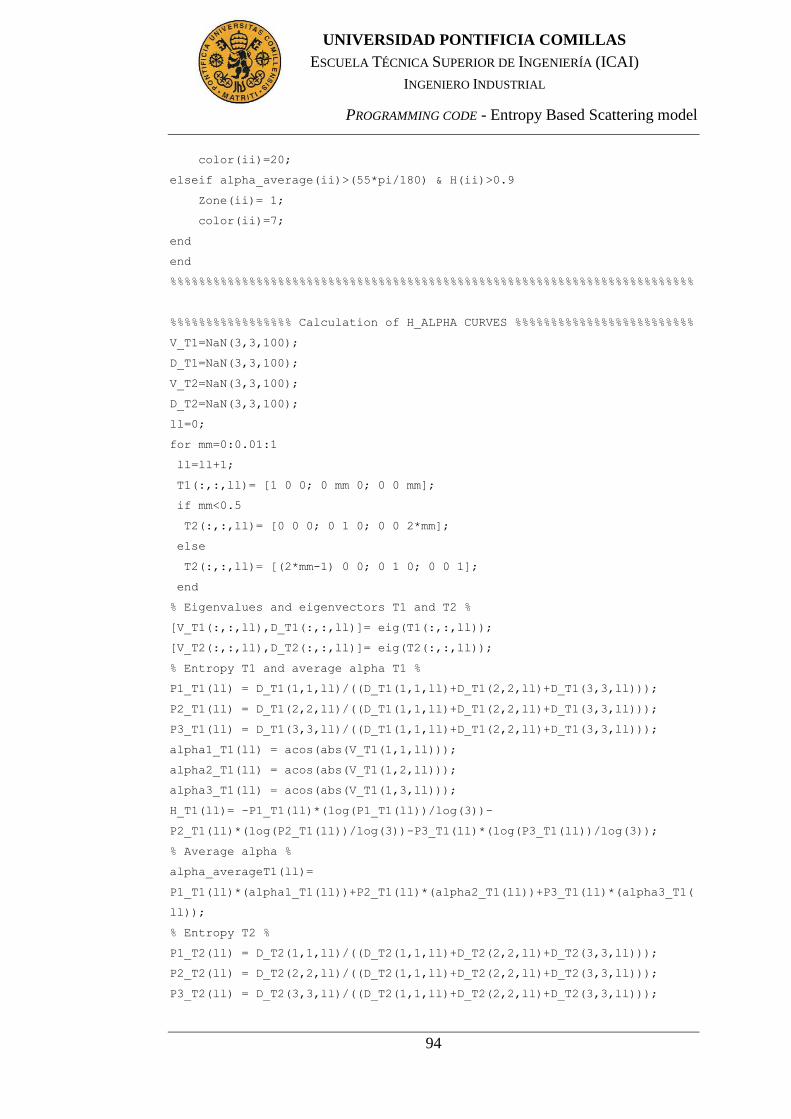
PROGRAMMING CODE - Entropy Based Scattering model
94
UNIVERSIDAD PONTIFICIA COMILLAS
ESCUELA TÉCNICA SUPERIOR DE INGENIERÍA (ICAI)
INGENIERO INDUSTRIAL
color(ii)=20;
elseif alpha_average(ii)>(55*pi/180) & H(ii)>0.9
Zone(ii)= 1;
color(ii)=7;
end
end
%%%%%%%%%%%%%%%%%%%%%%%%%%%%%%%%%%%%%%%%%%%%%%%%%%%%%%%%%%%%%%%%%%%%%%%%%
%%%%%%%%%%%%%%%%% Calculation of H_ALPHA CURVES %%%%%%%%%%%%%%%%%%%%%%%%%
V_T1=NaN(3,3,100);
D_T1=NaN(3,3,100);
V_T2=NaN(3,3,100);
D_T2=NaN(3,3,100);
ll=0;
for mm=0:0.01:1
ll=ll+1;
T1(:,:,ll)= [1 0 0; 0 mm 0; 0 0 mm];
if mm<0.5
T2(:,:,ll)= [0 0 0; 0 1 0; 0 0 2*mm];
else
T2(:,:,ll)= [(2*mm-1) 0 0; 0 1 0; 0 0 1];
end
% Eigenvalues and eigenvectors T1 and T2 %
[V_T1(:,:,ll),D_T1(:,:,ll)]= eig(T1(:,:,ll));
[V_T2(:,:,ll),D_T2(:,:,ll)]= eig(T2(:,:,ll));
% Entropy T1 and average alpha T1 %
P1_T1(ll) = D_T1(1,1,ll)/((D_T1(1,1,ll)+D_T1(2,2,ll)+D_T1(3,3,ll)));
P2_T1(ll) = D_T1(2,2,ll)/((D_T1(1,1,ll)+D_T1(2,2,ll)+D_T1(3,3,ll)));
P3_T1(ll) = D_T1(3,3,ll)/((D_T1(1,1,ll)+D_T1(2,2,ll)+D_T1(3,3,ll)));
alpha1_T1(ll) = acos(abs(V_T1(1,1,ll)));
alpha2_T1(ll) = acos(abs(V_T1(1,2,ll)));
alpha3_T1(ll) = acos(abs(V_T1(1,3,ll)));
H_T1(ll)= -P1_T1(ll)*(log(P1_T1(ll))/log(3))-
P2_T1(ll)*(log(P2_T1(ll))/log(3))-P3_T1(ll)*(log(P3_T1(ll))/log(3));
% Average alpha %
alpha_averageT1(ll)=
P1_T1(ll)*(alpha1_T1(ll))+P2_T1(ll)*(alpha2_T1(ll))+P3_T1(ll)*(alpha3_T1(
ll));
% Entropy T2 %
P1_T2(ll) = D_T2(1,1,ll)/((D_T2(1,1,ll)+D_T2(2,2,ll)+D_T2(3,3,ll)));
P2_T2(ll) = D_T2(2,2,ll)/((D_T2(1,1,ll)+D_T2(2,2,ll)+D_T2(3,3,ll)));
P3_T2(ll) = D_T2(3,3,ll)/((D_T2(1,1,ll)+D_T2(2,2,ll)+D_T2(3,3,ll)));

PROGRAMMING CODE - Entropy Based Scattering model
95
UNIVERSIDAD PONTIFICIA COMILLAS
ESCUELA TÉCNICA SUPERIOR DE INGENIERÍA (ICAI)
INGENIERO INDUSTRIAL
alpha1_T2(ll) = acos(abs(V_T2(1,1,ll)));
alpha2_T2(ll) = acos(abs(V_T2(1,2,ll)));
alpha3_T2(ll) = acos(abs(V_T2(1,3,ll)));
H_T2(ll)= -P1_T2(ll)*(log(P1_T2(ll))/log(3))-
P2_T2(ll)*(log(P2_T2(ll))/log(3))-P3_T2(ll)*(log(P3_T2(ll))/log(3));
% Average alpha %
alpha_averageT2(ll)=
P1_T2(ll)*(alpha1_T2(ll))+P2_T2(ll)*(alpha2_T2(ll))+P3_T2(ll)*(alpha3_T2(
ll));
end
%%%%%%%%%%%%%%%%%%%%%%%%%%%%%%%%%%%%%%%%%%%%%%%%%%%%%%%%%%%%%%%%%%%%%%%%%
%%%%%%%%%%%% Calculation of MEAN H and ALPHA FOR EACH FIELD %%%%%%%%%%%%%
mean_P=zeros(26,2);
%%%%%%%%%%%%%%%%%%%%%%%%%% Field 4 (grass)%%%%%%%%%%%%%%%%%%%%%%%%%%%%%%%
y_pixels=260; % first pixel of the field in vertical direction %
image_H = reshape(abs(H(:)), 1024, 1024)';
image_alpha = reshape(alpha_average(:), 1024, 1024)';
for ysquare_pixels=1:70 % 70 is the number of pixels in y direction %
x_pixels=150; % first pixel of the field in horizontal direction %
for xsquare_pixels=1:70 % 70 is the number of pixels in x direction %
pixels_square_H_1(xsquare_pixels,ysquare_pixels) =
image_H(x_pixels,y_pixels);
pixels_square_alpha_1(xsquare_pixels,ysquare_pixels) =
image_alpha(x_pixels,y_pixels);
x_pixels=x_pixels+1;
end
y_pixels=y_pixels+1;
end
pixels_notsquare_H=reshape(pixels_square_H_1,1,4900);
pixels_notsquare_alpha=reshape(pixels_square_alpha_1,1,4900);
mean_P(1,1)=mean(pixels_notsquare_H);
mean_P(1,2)=mean(pixels_notsquare_alpha);
%%%%%%%%%%%%%%%%%%%%%%%%%%%%%%%%%%%%%%%%%%%%%%%%%%%%%%%%%%%%%%%%%%%%%%%%%
%%%%%%%%%%%%%%%%%%%%%%%% Field 30 (beets)% %%%%%%%%%%%%%%%%%%%%%%%%%%%%%%
y_pixels=70; % first pixel of the field in vertical direction %
image_H = reshape(abs(H(:)), 1024, 1024)';
image_alpha = reshape(alpha_average(:), 1024, 1024)';

PROGRAMMING CODE - Entropy Based Scattering model
96
UNIVERSIDAD PONTIFICIA COMILLAS
ESCUELA TÉCNICA SUPERIOR DE INGENIERÍA (ICAI)
INGENIERO INDUSTRIAL
for ysquare_pixels=1:15 % 15 is the number of pixels in y direction %
x_pixels=260; % first pixel of the field in horizontal direction %
for xsquare_pixels=1:15 % 15 is the number of pixels in x direction %
pixels_square_H_2(xsquare_pixels,ysquare_pixels) =
image_H(x_pixels,y_pixels);
pixels_square_alpha_2(xsquare_pixels,ysquare_pixels) =
image_alpha(x_pixels,y_pixels);
x_pixels=x_pixels+1;
end
y_pixels=y_pixels+1;
end
pixels_notsquare_H=reshape(pixels_square_H_2,1,225);
pixels_notsquare_alpha=reshape(pixels_square_alpha_2,1,225);
mean_P(2,1)=mean(pixels_notsquare_H);
mean_P(2,2)=mean(pixels_notsquare_alpha);
%%%%%%%%%%%%%%%%%%%%%%%%%%%%%%%%%%%%%%%%%%%%%%%%%%%%%%%%%%%%%%%%%%%%%%%%%
%%%%%%%%%%%%%%%%%%%%%%%% Field 3 (winter wheat) %%%%%%%%%%%%%%%%%%%%%%%%%
y_pixels=195; % first pixel of the field in vertical direction %
image_H = reshape(abs(H(:)), 1024, 1024)';
image_alpha = reshape(alpha_average(:), 1024, 1024)';
for ysquare_pixels=1:30 % 30 is the number of pixels in y direction %
x_pixels=250;
for xsquare_pixels=1:30 % 30 is the number of pixels in x direction %
pixels_square_H_3(xsquare_pixels,ysquare_pixels) =
image_H(x_pixels,y_pixels);
pixels_square_alpha_3(xsquare_pixels,ysquare_pixels) =
image_alpha(x_pixels,y_pixels);
x_pixels=x_pixels+1;
end
y_pixels=y_pixels+1;
end
pixels_notsquare_H=reshape(pixels_square_H_3,1,900);
pixels_notsquare_alpha=reshape(pixels_square_alpha_3,1,900);
mean_P(3,1)=mean(pixels_notsquare_H);
mean_P(3,2)=mean(pixels_notsquare_alpha);
%%%%%%%%%%%%%%%%%%%%%%%%%%%%%%%%%%%%%%%%%%%%%%%%%%%%%%%%%%%%%%%%%%%%%%%%%
%%%%%%%%%%%%%%%%%%%%%%%% Field 5 (winter wheat)% %%%%%%%%%%%%%%%%%%%%%%%%
y_pixels=340; % first pixel of the field in vertical direction %
image_H = reshape(abs(H(:)), 1024, 1024)';
image_alpha = reshape(alpha_average(:), 1024, 1024)';

PROGRAMMING CODE - Entropy Based Scattering model
97
UNIVERSIDAD PONTIFICIA COMILLAS
ESCUELA TÉCNICA SUPERIOR DE INGENIERÍA (ICAI)
INGENIERO INDUSTRIAL
for ysquare_pixels=1:70 % 70 is the number of pixels in y direction %
x_pixels=220;
for xsquare_pixels=1:70 % 70 is the number of pixels in x direction %
pixels_square_H_4(xsquare_pixels,ysquare_pixels) =
image_H(x_pixels,y_pixels);
pixels_square_alpha_4(xsquare_pixels,ysquare_pixels) =
image_alpha(x_pixels,y_pixels);
x_pixels=x_pixels+1;
end
y_pixels=y_pixels+1;
end
pixels_notsquare_H=reshape(pixels_square_H_4,1,4900);
pixels_notsquare_alpha=reshape(pixels_square_alpha_4,1,4900);
mean_P(4,1)=mean(pixels_notsquare_H);
mean_P(4,2)=mean(pixels_notsquare_alpha);
%%%%%%%%%%%%%%%%%%%%%%%%%%%%%%%%%%%%%%%%%%%%%%%%%%%%%%%%%%%%%%%%%%%%%%%%%
%%%%%%%%%%%%%%%%%%%%%%%% Field 11 (winter wheat) %%%%%%%%%%%%%%%%%%%%%%%%
y_pixels=540; % first pixel of the field in vertical direction %
image_H = reshape(abs(H(:)), 1024, 1024)';
image_alpha = reshape(alpha_average(:), 1024, 1024)';
for ysquare_pixels=1:60 % 60 is the number of pixels in y direction %
x_pixels=420;
for xsquare_pixels=1:60 % 60 is the number of pixels in x direction %
pixels_square_H_5(xsquare_pixels,ysquare_pixels) =
image_H(x_pixels,y_pixels);
pixels_square_alpha_5(xsquare_pixels,ysquare_pixels) =
image_alpha(x_pixels,y_pixels);
x_pixels=x_pixels+1;
end
y_pixels=y_pixels+1;
end
pixels_notsquare_H=reshape(pixels_square_H_5,1,3600);
pixels_notsquare_alpha=reshape(pixels_square_alpha_5,1,3600);
mean_P(5,1)=mean(pixels_notsquare_H);
mean_P(5,2)=mean(pixels_notsquare_alpha);
%%%%%%%%%%%%%%%%%%%%%%%%%%%%%%%%%%%%%%%%%%%%%%%%%%%%%%%%%%%%%%%%%%%%%%%%%
%%%%%%%%%%%%%%%%%%%%%% Field 20 (winter wheat)%%%%%%%%%%%%%%%%%%%%%%%%%%%
y_pixels=585; % first pixel of the field in vertical direction %
image_H = reshape(abs(H(:)), 1024, 1024)';

PROGRAMMING CODE - Entropy Based Scattering model
98
UNIVERSIDAD PONTIFICIA COMILLAS
ESCUELA TÉCNICA SUPERIOR DE INGENIERÍA (ICAI)
INGENIERO INDUSTRIAL
image_alpha = reshape(alpha_average(:), 1024, 1024)';
for ysquare_pixels=1:40 % 40 is the number of pixels in y direction %
x_pixels=785;
for xsquare_pixels=1:40 % 40 is the number of pixels in x direction %
pixels_square_H_6(xsquare_pixels,ysquare_pixels) =
image_H(x_pixels,y_pixels);
pixels_square_alpha_6(xsquare_pixels,ysquare_pixels) =
image_alpha(x_pixels,y_pixels);
x_pixels=x_pixels+1;
end
y_pixels=y_pixels+1;
end
pixels_notsquare_H=reshape(pixels_square_H_6,1,1600);
pixels_notsquare_alpha=reshape(pixels_square_alpha_6,1,1600);
mean_P(6,1)=mean(pixels_notsquare_H);
mean_P(6,2)=mean(pixels_notsquare_alpha);
%%%%%%%%%%%%%%%%%%%%%%%%%%%%%%%%%%%%%%%%%%%%%%%%%%%%%%%%%%%%%%%%%%%%%%%%%
%%%%%%%%%%%%%%%%%%%%%%%% Field 27 (winter wheat)% %%%%%%%%%%%%%%%%%%%%%%%
y_pixels=970; % first pixel of the field in vertical direction %
image_H = reshape(abs(H(:)), 1024, 1024)';
image_alpha = reshape(alpha_average(:), 1024, 1024)';
for ysquare_pixels=1:40 % 40 is the number of pixels in y direction %
x_pixels=690;
for xsquare_pixels=1:40 % 40 is the number of pixels in x direction %
pixels_square_H_7(xsquare_pixels,ysquare_pixels) =
image_H(x_pixels,y_pixels);
pixels_square_alpha_7(xsquare_pixels,ysquare_pixels) =
image_alpha(x_pixels,y_pixels);
x_pixels=x_pixels+1;
end
y_pixels=y_pixels+1;
end
pixels_notsquare_H=reshape(pixels_square_H_7,1,1600);
pixels_notsquare_alpha=reshape(pixels_square_alpha_7,1,1600);
mean_P(7,1)=mean(pixels_notsquare_H);
mean_P(7,2)=mean(pixels_notsquare_alpha);
%%%%%%%%%%%%%%%%%%%%%%%%%%%%%%%%%%%%%%%%%%%%%%%%%%%%%%%%%%%%%%%%%%%%%%%%%
%%%%%%%%%%%%%%%%%%%%%% Field 33 (winter wheat)% %%%%%%%%%%%%%%%%%%%%%%%%%
y_pixels=75; % first pixel of the field in vertical direction %
image_H = reshape(abs(H(:)), 1024, 1024)';

PROGRAMMING CODE - Entropy Based Scattering model
99
UNIVERSIDAD PONTIFICIA COMILLAS
ESCUELA TÉCNICA SUPERIOR DE INGENIERÍA (ICAI)
INGENIERO INDUSTRIAL
image_alpha = reshape(alpha_average(:), 1024, 1024)';
for ysquare_pixels=1:30 % 30 is the number of pixels in y direction %
x_pixels=90;
for xsquare_pixels=1:30 % 30 is the number of pixels in x direction %
pixels_square_H_8(xsquare_pixels,ysquare_pixels) =
image_H(x_pixels,y_pixels);
pixels_square_alpha_8(xsquare_pixels,ysquare_pixels) =
image_alpha(x_pixels,y_pixels);
x_pixels=x_pixels+1;
end
y_pixels=y_pixels+1;
end
pixels_notsquare_H=reshape(pixels_square_H_8,1,900);
pixels_notsquare_alpha=reshape(pixels_square_alpha_8,1,900);
mean_P(8,1)=mean(pixels_notsquare_H);
mean_P(8,2)=mean(pixels_notsquare_alpha);
%%%%%%%%%%%%%%%%%%%%%%%%%%%%%%%%%%%%%%%%%%%%%%%%%%%%%%%%%%%%%%%%%%%%%%%%%
%%%%%%%%%%%%%%%%%%%%%%% Field 6 (spring barley) %%%%%%%%%%%%%%%%%%%%%%%%%
y_pixels=450; % first pixel of the field in vertical direction %
image_H = reshape(abs(H(:)), 1024, 1024)';
image_alpha = reshape(alpha_average(:), 1024, 1024)';
for ysquare_pixels=1:50 % 50 is the number of pixels in y direction %
x_pixels=230;
for xsquare_pixels=1:50 % 50 is the number of pixels in x direction %
pixels_square_H_9(xsquare_pixels,ysquare_pixels) =
image_H(x_pixels,y_pixels);
pixels_square_alpha_9(xsquare_pixels,ysquare_pixels) =
image_alpha(x_pixels,y_pixels);
x_pixels=x_pixels+1;
end
y_pixels=y_pixels+1;
end
pixels_notsquare_H=reshape(pixels_square_H_9,1,2500);
pixels_notsquare_alpha=reshape(pixels_square_alpha_9,1,2500);
mean_P(9,1)=mean(pixels_notsquare_H);
mean_P(9,2)=mean(pixels_notsquare_alpha);
%%%%%%%%%%%%%%%%%%%%%%%%%%%%%%%%%%%%%%%%%%%%%%%%%%%%%%%%%%%%%%%%%%%%%%%%%
%%%%%%%%%%%%%%%%%%%%%% Field 13 (spring barley) %%%%%%%%%%%%%%%%%%%%%%%%%
y_pixels=728; % first pixel of the field in vertical direction %
image_H = reshape(abs(H(:)), 1024, 1024)';

PROGRAMMING CODE - Entropy Based Scattering model
100
UNIVERSIDAD PONTIFICIA COMILLAS
ESCUELA TÉCNICA SUPERIOR DE INGENIERÍA (ICAI)
INGENIERO INDUSTRIAL
image_alpha = reshape(alpha_average(:), 1024, 1024)';
for ysquare_pixels=1:30 % 30 is the number of pixels in y direction %
x_pixels=428;
for xsquare_pixels=1:30 % 30 is the number of pixels in x direction %
pixels_square_H_10(xsquare_pixels,ysquare_pixels) =
image_H(x_pixels,y_pixels);
pixels_square_alpha_10(xsquare_pixels,ysquare_pixels) =
image_alpha(x_pixels,y_pixels);
x_pixels=x_pixels+1;
end
y_pixels=y_pixels+1;
end
pixels_notsquare_H=reshape(pixels_square_H_10,1,900);
pixels_notsquare_alpha=reshape(pixels_square_alpha_10,1,900);
mean_P(10,1)=mean(pixels_notsquare_H);
mean_P(10,2)=mean(pixels_notsquare_alpha);
%%%%%%%%%%%%%%%%%%%%%%%%%%%%%%%%%%%%%%%%%%%%%%%%%%%%%%%%%%%%%%%%%%%%%%%%%
%%%%%%%%%%%%%%%%%%%%% Field 14 (spring barley) %%%%%%%%%%%%%%%%%%%%%%%%%%
y_pixels=700; % first pixel of the field in vertical direction %
image_H = reshape(abs(H(:)), 1024, 1024)';
image_alpha = reshape(alpha_average(:), 1024, 1024)';
for ysquare_pixels=1:10 % 10 is the number of pixels in y direction %
x_pixels=490;
for xsquare_pixels=1:10 % 10 is the number of pixels in x direction %
pixels_square_H_11(xsquare_pixels,ysquare_pixels) =
image_H(x_pixels,y_pixels);
pixels_square_alpha_11(xsquare_pixels,ysquare_pixels) =
image_alpha(x_pixels,y_pixels);
x_pixels=x_pixels+1;
end
y_pixels=y_pixels+1;
end
pixels_notsquare_H=reshape(pixels_square_H_11,1,100);
pixels_notsquare_alpha=reshape(pixels_square_alpha_11,1,100);
mean_P(11,1)=mean(pixels_notsquare_H);
mean_P(11,2)=mean(pixels_notsquare_alpha);
%%%%%%%%%%%%%%%%%%%%%%%%%%%%%%%%%%%%%%%%%%%%%%%%%%%%%%%%%%%%%%%%%%%%%%%%%
%%%%%%%%%%%%%%%%%%%%%% Field 29 (spring barley) %%%%%%%%%%%%%%%%%%%%%%%%%
y_pixels=90;
image_H = reshape(abs(H(:)), 1024, 1024)';

PROGRAMMING CODE - Entropy Based Scattering model
101
UNIVERSIDAD PONTIFICIA COMILLAS
ESCUELA TÉCNICA SUPERIOR DE INGENIERÍA (ICAI)
INGENIERO INDUSTRIAL
image_alpha = reshape(alpha_average(:), 1024, 1024)';
for ysquare_pixels=1:10 % 10 is the number of pixels in y direction %
x_pixels=275;
for xsquare_pixels=1:10 % 10 is the number of pixels in x direction %
pixels_square_H_12(xsquare_pixels,ysquare_pixels) =
image_H(x_pixels,y_pixels);
pixels_square_alpha_12(xsquare_pixels,ysquare_pixels) =
image_alpha(x_pixels,y_pixels);
x_pixels=x_pixels+1;
end
y_pixels=y_pixels+1;
end
pixels_notsquare_H=reshape(pixels_square_H_12,1,100);
pixels_notsquare_alpha=reshape(pixels_square_alpha_12,1,100);
mean_P(12,1)=mean(pixels_notsquare_H);
mean_P(12,2)=mean(pixels_notsquare_alpha);
%%%%%%%%%%%%%%%%%%%%%%%%%%%%%%%%%%%%%%%%%%%%%%%%%%%%%%%%%%%%%%%%%%%%%%%%%
%%%%%%%%%%%%%%%%%%%%%%%% Field 31 (spring barley) %%%%%%%%%%%%%%%%%%%%%%%
y_pixels=40; % first pixel of the field in vertical direction %
image_H = reshape(abs(H(:)), 1024, 1024)';
image_alpha = reshape(alpha_average(:), 1024, 1024)';
for ysquare_pixels=1:20 % 20 is the number of pixels in y direction %
x_pixels=245;
for xsquare_pixels=1:20 % 20 is the number of pixels in x direction %
pixels_square_H_13(xsquare_pixels,ysquare_pixels) =
image_H(x_pixels,y_pixels);
pixels_square_alpha_13(xsquare_pixels,ysquare_pixels) =
image_alpha(x_pixels,y_pixels);
x_pixels=x_pixels+1;
end
y_pixels=y_pixels+1;
end
pixels_notsquare_H=reshape(pixels_square_H_13,1,400);
pixels_notsquare_alpha=reshape(pixels_square_alpha_13,1,400);
mean_P(13,1)=mean(pixels_notsquare_H);
mean_P(13,2)=mean(pixels_notsquare_alpha);
%%%%%%%%%%%%%%%%%%%%%%%%%%%%%%%%%%%%%%%%%%%%%%%%%%%%%%%%%%%%%%%%%%%%%%%%%
%%%%%%%%%%%%%%%%%%%% Field 34 (spring barley)% %%%%%%%%%%%%%%%%%%%%%%%%%%
y_pixels=130; % first pixel of the field in vertical direction %
image_H = reshape(abs(H(:)), 1024, 1024)';

PROGRAMMING CODE - Entropy Based Scattering model
102
UNIVERSIDAD PONTIFICIA COMILLAS
ESCUELA TÉCNICA SUPERIOR DE INGENIERÍA (ICAI)
INGENIERO INDUSTRIAL
image_alpha = reshape(alpha_average(:), 1024, 1024)';
for ysquare_pixels=1:15 % 15 is the number of pixels in y direction %
x_pixels=110;
for xsquare_pixels=1:15 % 15 is the number of pixels in x direction %
pixels_square_H_14(xsquare_pixels,ysquare_pixels) =
image_H(x_pixels,y_pixels);
pixels_square_alpha_14(xsquare_pixels,ysquare_pixels) =
image_alpha(x_pixels,y_pixels);
x_pixels=x_pixels+1;
end
y_pixels=y_pixels+1;
end
pixels_notsquare_H=reshape(pixels_square_H_14,1,225);
pixels_notsquare_alpha=reshape(pixels_square_alpha_14,1,225);
mean_P(14,1)=mean(pixels_notsquare_H);
mean_P(14,2)=mean(pixels_notsquare_alpha);
%%%%%%%%%%%%%%%%%%%%%%%%%%%%%%%%%%%%%%%%%%%%%%%%%%%%%%%%%%%%%%%%%%%%%%%%%
%%%%%%%%%%%%%%%%%%%%% Field 36 (spring barley)% %%%%%%%%%%%%%%%%%%%%%%%%%
y_pixels=150; % first pixel of the field in vertical direction %
image_H = reshape(abs(H(:)), 1024, 1024)';
image_alpha = reshape(alpha_average(:), 1024, 1024)';
for ysquare_pixels=1:30 % 30 is the number of pixels in y direction %
x_pixels=50;
for xsquare_pixels=1:30 % 30 is the number of pixels in x direction %
pixels_square_H_15(xsquare_pixels,ysquare_pixels) =
image_H(x_pixels,y_pixels);
pixels_square_alpha_15(xsquare_pixels,ysquare_pixels) =
image_alpha(x_pixels,y_pixels);
x_pixels=x_pixels+1;
end
y_pixels=y_pixels+1;
end
pixels_notsquare_H=reshape(pixels_square_H_15,1,900);
pixels_notsquare_alpha=reshape(pixels_square_alpha_15,1,900);
mean_P(15,1)=mean(pixels_notsquare_H);
mean_P(15,2)=mean(pixels_notsquare_alpha);
%%%%%%%%%%%%%%%%%%%%%%%%%%%%%%%%%%%%%%%%%%%%%%%%%%%%%%%%%%%%%%%%%%%%%%%%%
%%%%%%%%%%%%%%%%%%%%%%%%%% Field 1 (Rye)% %%%%%%%%%%%%%%%%%%%%%%%%%%%%%%%
y_pixels=115; % first pixel of the field in vertical direction %
image_H = reshape(abs(H(:)), 1024, 1024)';

PROGRAMMING CODE - Entropy Based Scattering model
103
UNIVERSIDAD PONTIFICIA COMILLAS
ESCUELA TÉCNICA SUPERIOR DE INGENIERÍA (ICAI)
INGENIERO INDUSTRIAL
image_alpha = reshape(alpha_average(:), 1024, 1024)';
for ysquare_pixels=1:40 % 40 is the number of pixels in y direction %
x_pixels=335;
for xsquare_pixels=1:40 % 40 is the number of pixels in x direction %
pixels_square_H_16(xsquare_pixels,ysquare_pixels) =
image_H(x_pixels,y_pixels);
pixels_square_alpha_16(xsquare_pixels,ysquare_pixels) =
image_alpha(x_pixels,y_pixels);
x_pixels=x_pixels+1;
end
y_pixels=y_pixels+1;
end
pixels_notsquare_H=reshape(pixels_square_H_16,1,1600);
pixels_notsquare_alpha=reshape(pixels_square_alpha_16,1,1600);
mean_P(16,1)=mean(pixels_notsquare_H);
mean_P(16,2)=mean(pixels_notsquare_alpha);
%%%%%%%%%%%%%%%%%%%%%%%%%%%%%%%%%%%%%%%%%%%%%%%%%%%%%%%%%%%%%%%%%%%%%%%%%
%%%%%%%%%%%%%%%%%%%%%%%%%%% Field 8 (Rye) %%%%%%%%%%%%%%%%%%%%%%%%%%%%%%%
y_pixels=355; % first pixel of the field in vertical direction %
image_H = reshape(abs(H(:)), 1024, 1024)';
image_alpha = reshape(alpha_average(:), 1024, 1024)';
for ysquare_pixels=1:70 % 70 is the number of pixels in y direction %
x_pixels=360;
for xsquare_pixels=1:70 % 70 is the number of pixels in x direction %
pixels_square_H_17(xsquare_pixels,ysquare_pixels) =
image_H(x_pixels,y_pixels);
pixels_square_alpha_17(xsquare_pixels,ysquare_pixels) =
image_alpha(x_pixels,y_pixels);
x_pixels=x_pixels+1;
end
y_pixels=y_pixels+1;
end
pixels_notsquare_H=reshape(pixels_square_H_17,1,4900);
pixels_notsquare_alpha=reshape(pixels_square_alpha_17,1,4900);
mean_P(17,1)=mean(pixels_notsquare_H);
mean_P(17,2)=mean(pixels_notsquare_alpha);
%%%%%%%%%%%%%%%%%%%%%%%%%%%%%%%%%%%%%%%%%%%%%%%%%%%%%%%%%%%%%%%%%%%%%%%%%
%%%%%%%%%%%%%%%%%%%%%%%%%%% Field 12 (Rye)%%%%%%%%%%%%%%%%%%%%%%%%%%%%%%%
y_pixels=700; % first pixel of the field in vertical direction %
image_H = reshape(abs(H(:)), 1024, 1024)';

PROGRAMMING CODE - Entropy Based Scattering model
104
UNIVERSIDAD PONTIFICIA COMILLAS
ESCUELA TÉCNICA SUPERIOR DE INGENIERÍA (ICAI)
INGENIERO INDUSTRIAL
image_alpha = reshape(alpha_average(:), 1024, 1024)';
for ysquare_pixels=1:60 % 60 is the number of pixels in y direction %
x_pixels=340;
for xsquare_pixels=1:60 % 60 is the number of pixels in x direction %
pixels_square_H_18(xsquare_pixels,ysquare_pixels) =
image_H(x_pixels,y_pixels);
pixels_square_alpha_18(xsquare_pixels,ysquare_pixels) =
image_alpha(x_pixels,y_pixels);
x_pixels=x_pixels+1;
end
y_pixels=y_pixels+1;
end
pixels_notsquare_H=reshape(pixels_square_H_18,1,3600);
pixels_notsquare_alpha=reshape(pixels_square_alpha_18,1,3600);
mean_P(18,1)=mean(pixels_notsquare_H);
mean_P(18,2)=mean(pixels_notsquare_alpha);
%%%%%%%%%%%%%%%%%%%%%%%%%%%%%%%%%%%%%%%%%%%%%%%%%%%%%%%%%%%%%%%%%%%%%%%%%
%%%%%%%%%%%%%%%%%%%%%%%%%%%% Field 23 (Rye)%%%%%%%%%%%%%%%%%%%%%%%%%%%%%%
y_pixels=810; % first pixel of the field in vertical direction %
image_H = reshape(abs(H(:)), 1024, 1024)';
image_alpha = reshape(alpha_average(:), 1024, 1024)';
for ysquare_pixels=1:70 % 70 is the number of pixels in y direction %
x_pixels=690;
for xsquare_pixels=1:70 % 70 is the number of pixels in x direction %
pixels_square_H_19(xsquare_pixels,ysquare_pixels) =
image_H(x_pixels,y_pixels);
pixels_square_alpha_19(xsquare_pixels,ysquare_pixels) =
image_alpha(x_pixels,y_pixels);
x_pixels=x_pixels+1;
end
y_pixels=y_pixels+1;
end
pixels_notsquare_H=reshape(pixels_square_H_19,1,4900);
pixels_notsquare_alpha=reshape(pixels_square_alpha_19,1,4900);
mean_P(19,1)=mean(pixels_notsquare_H);
mean_P(19,2)=mean(pixels_notsquare_alpha);
%%%%%%%%%%%%%%%%%%%%%%%%%%%%%%%%%%%%%%%%%%%%%%%%%%%%%%%%%%%%%%%%%%%%%%%%%
%%%%%%%%%%%%%%%%%%%%%%%%%%%% Field 7 (Peas)% %%%%%%%%%%%%%%%%%%%%%%%%%%%%
y_pixels=295; % first pixel of the field in vertical direction %
image_H = reshape(abs(H(:)), 1024, 1024)';

PROGRAMMING CODE - Entropy Based Scattering model
105
UNIVERSIDAD PONTIFICIA COMILLAS
ESCUELA TÉCNICA SUPERIOR DE INGENIERÍA (ICAI)
INGENIERO INDUSTRIAL
image_alpha = reshape(alpha_average(:), 1024, 1024)';
for ysquare_pixels=1:15 % 15 is the number of pixels in y direction %
x_pixels=395;
for xsquare_pixels=1:15 % 15 is the number of pixels in x direction %
pixels_square_H_20(xsquare_pixels,ysquare_pixels) =
image_H(x_pixels,y_pixels);
pixels_square_alpha_20(xsquare_pixels,ysquare_pixels) =
image_alpha(x_pixels,y_pixels);
x_pixels=x_pixels+1;
end
y_pixels=y_pixels+1;
end
pixels_notsquare_H=reshape(pixels_square_H_20,1,225);
pixels_notsquare_alpha=reshape(pixels_square_alpha_20,1,225);
mean_P(20,1)=mean(pixels_notsquare_H);
mean_P(20,2)=mean(pixels_notsquare_alpha);
%%%%%%%%%%%%%%%%%%%%%%%%%%%%%%%%%%%%%%%%%%%%%%%%%%%%%%%%%%%%%%%%%%%%%%%%%
%%%%%%%%%%%%%%%%%%%%%%%%%%% Field 15 (Peas)% %%%%%%%%%%%%%%%%%%%%%%%%%%%%
y_pixels=730; % first pixel of the field in vertical direction %
image_H = reshape(abs(H(:)), 1024, 1024)';
image_alpha = reshape(alpha_average(:), 1024, 1024)';
for ysquare_pixels=1:70 % 70 is the number of pixels in y direction %
x_pixels=575;
for xsquare_pixels=1:70 % 70 is the number of pixels in x direction %
pixels_square_H_21(xsquare_pixels,ysquare_pixels) =
image_H(x_pixels,y_pixels);
pixels_square_alpha_21(xsquare_pixels,ysquare_pixels) =
image_alpha(x_pixels,y_pixels);
x_pixels=x_pixels+1;
end
y_pixels=y_pixels+1;
end
pixels_notsquare_H=reshape(pixels_square_H_21,1,4900);
pixels_notsquare_alpha=reshape(pixels_square_alpha_21,1,4900);
mean_P(21,1)=mean(pixels_notsquare_H);
mean_P(21,2)=mean(pixels_notsquare_alpha);
%%%%%%%%%%%%%%%%%%%%%%%%%%%%%%%%%%%%%%%%%%%%%%%%%%%%%%%%%%%%%%%%%%%%%%%%%
&&&&%%%%%%%%%%%%%%%%%%%%%% Field 18 (Peas)% %%%%%%%%%%%%%%%%%%%%%%%%%%%%%
y_pixels=555;
image_H = reshape(abs(H(:)), 1024, 1024)';
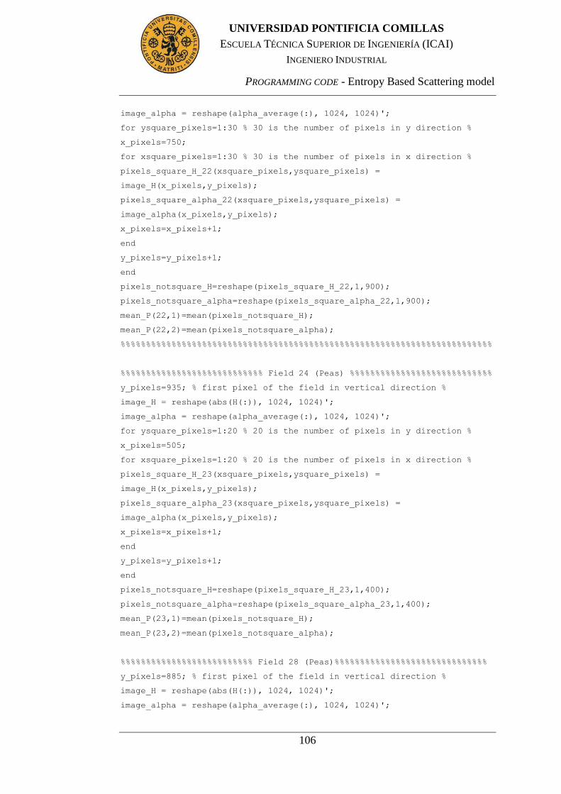
PROGRAMMING CODE - Entropy Based Scattering model
106
UNIVERSIDAD PONTIFICIA COMILLAS
ESCUELA TÉCNICA SUPERIOR DE INGENIERÍA (ICAI)
INGENIERO INDUSTRIAL
image_alpha = reshape(alpha_average(:), 1024, 1024)';
for ysquare_pixels=1:30 % 30 is the number of pixels in y direction %
x_pixels=750;
for xsquare_pixels=1:30 % 30 is the number of pixels in x direction %
pixels_square_H_22(xsquare_pixels,ysquare_pixels) =
image_H(x_pixels,y_pixels);
pixels_square_alpha_22(xsquare_pixels,ysquare_pixels) =
image_alpha(x_pixels,y_pixels);
x_pixels=x_pixels+1;
end
y_pixels=y_pixels+1;
end
pixels_notsquare_H=reshape(pixels_square_H_22,1,900);
pixels_notsquare_alpha=reshape(pixels_square_alpha_22,1,900);
mean_P(22,1)=mean(pixels_notsquare_H);
mean_P(22,2)=mean(pixels_notsquare_alpha);
%%%%%%%%%%%%%%%%%%%%%%%%%%%%%%%%%%%%%%%%%%%%%%%%%%%%%%%%%%%%%%%%%%%%%%%%%
%%%%%%%%%%%%%%%%%%%%%%%%%%%% Field 24 (Peas) %%%%%%%%%%%%%%%%%%%%%%%%%%%%
y_pixels=935; % first pixel of the field in vertical direction %
image_H = reshape(abs(H(:)), 1024, 1024)';
image_alpha = reshape(alpha_average(:), 1024, 1024)';
for ysquare_pixels=1:20 % 20 is the number of pixels in y direction %
x_pixels=505;
for xsquare_pixels=1:20 % 20 is the number of pixels in x direction %
pixels_square_H_23(xsquare_pixels,ysquare_pixels) =
image_H(x_pixels,y_pixels);
pixels_square_alpha_23(xsquare_pixels,ysquare_pixels) =
image_alpha(x_pixels,y_pixels);
x_pixels=x_pixels+1;
end
y_pixels=y_pixels+1;
end
pixels_notsquare_H=reshape(pixels_square_H_23,1,400);
pixels_notsquare_alpha=reshape(pixels_square_alpha_23,1,400);
mean_P(23,1)=mean(pixels_notsquare_H);
mean_P(23,2)=mean(pixels_notsquare_alpha);
%%%%%%%%%%%%%%%%%%%%%%%%%% Field 28 (Peas)%%%%%%%%%%%%%%%%%%%%%%%%%%%%%%
y_pixels=885; % first pixel of the field in vertical direction %
image_H = reshape(abs(H(:)), 1024, 1024)';
image_alpha = reshape(alpha_average(:), 1024, 1024)';

PROGRAMMING CODE - Entropy Based Scattering model
107
UNIVERSIDAD PONTIFICIA COMILLAS
ESCUELA TÉCNICA SUPERIOR DE INGENIERÍA (ICAI)
INGENIERO INDUSTRIAL
for ysquare_pixels=1:30 % 30 is the number of pixels in y direction %
x_pixels=835;
for xsquare_pixels=1:30 % 30 is the number of pixels in x direction %
pixels_square_H_24(xsquare_pixels,ysquare_pixels) =
image_H(x_pixels,y_pixels);
pixels_square_alpha_24(xsquare_pixels,ysquare_pixels) =
image_alpha(x_pixels,y_pixels);
x_pixels=x_pixels+1;
end
y_pixels=y_pixels+1;
end
pixels_notsquare_H=reshape(pixels_square_H_24,1,900);
pixels_notsquare_alpha=reshape(pixels_square_alpha_24,1,900);
mean_P(24,1)=mean(pixels_notsquare_H);
mean_P(24,2)=mean(pixels_notsquare_alpha);
%%%%%%%%%%%%%%%%%%%%%%%%%%%%%%%%%%%%%%%%%%%%%%%%%%%%%%%%%%%%%%%%%%%%%%%%%
%%%%%%%%%%%%%%%%%%%%%%%%%%%%% Field 37 (Peas)%%%%%%%%%%%%%%%%%%%%%%%%%%%%
y_pixels=215; % first pixel of the field in vertical direction %
image_H = reshape(abs(H(:)), 1024, 1024)';
image_alpha = reshape(alpha_average(:), 1024, 1024)';
for ysquare_pixels=1:20 % 20 is the number of pixels in y direction %
x_pixels=45;
for xsquare_pixels=1:20 % 20 is the number of pixels in x direction %
pixels_square_H_25(xsquare_pixels,ysquare_pixels) =
image_H(x_pixels,y_pixels);
pixels_square_alpha_25(xsquare_pixels,ysquare_pixels) =
image_alpha(x_pixels,y_pixels);
x_pixels=x_pixels+1;
end
y_pixels=y_pixels+1;
end
pixels_notsquare_H=reshape(pixels_square_H_25,1,400);
pixels_notsquare_alpha=reshape(pixels_square_alpha_25,1,400);
mean_P(25,1)=mean(pixels_notsquare_H);
mean_P(25,2)=mean(pixels_notsquare_alpha);
%%%%%%%%%%%%%%%%%%%%%%%%%%%%%%%%%%%%%%%%%%%%%%%%%%%%%%%%%%%%%%%%%%%%%%%%%
%%%%%%%%%%%%%%%%%%%%%%%% Field 9 (Spring oats)%%%%%%%%%%%%%%%%%%%%%%%%%%%
y_pixels=450; % first pixel of the field in vertical direction %
image_H = reshape(abs(H(:)), 1024, 1024)';
image_alpha = reshape(alpha_average(:), 1024, 1024)';

PROGRAMMING CODE - Entropy Based Scattering model
108
UNIVERSIDAD PONTIFICIA COMILLAS
ESCUELA TÉCNICA SUPERIOR DE INGENIERÍA (ICAI)
INGENIERO INDUSTRIAL
for ysquare_pixels=1:40 % 40 is the number of pixels in y direction %
x_pixels=405; % first pixel of the field in vertical direction %
for xsquare_pixels=1:40 % 40 is the number of pixels in x direction %
pixels_square_H_26(xsquare_pixels,ysquare_pixels) =
image_H(x_pixels,y_pixels);
pixels_square_alpha_26(xsquare_pixels,ysquare_pixels) =
image_alpha(x_pixels,y_pixels);
x_pixels=x_pixels+1;
end
y_pixels=y_pixels+1;
end
pixels_notsquare_H=reshape(pixels_square_H_26,1,1600);
pixels_notsquare_alpha=reshape(pixels_square_alpha_26,1,1600);
mean_P(26,1)=mean(pixels_notsquare_H);
mean_P(26,2)=mean(pixels_notsquare_alpha);
%%%%%%%%%%%%%%%%%%%%%%%%%%%%%%%%%%%%%%%%%%%%%%%%%%%%%%%%%%%%%%%%%%%%%%%%%
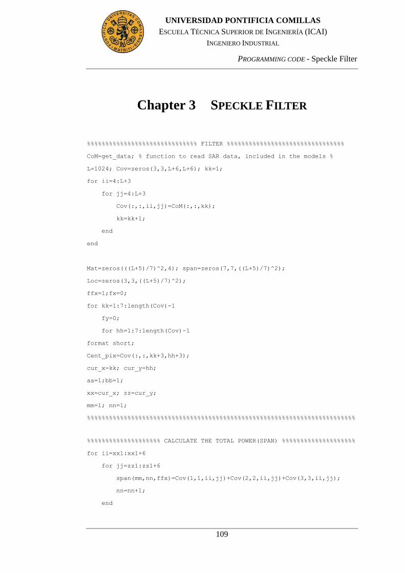
PROGRAMMING CODE - Speckle Filter
109
UNIVERSIDAD PONTIFICIA COMILLAS
ESCUELA TÉCNICA SUPERIOR DE INGENIERÍA (ICAI)
INGENIERO INDUSTRIAL
Chapter 3 SPECKLE FILTER
%%%%%%%%%%%%%%%%%%%%%%%%%%%%%% FILTER %%%%%%%%%%%%%%%%%%%%%%%%%%%%%%%%
CoM=get_data; % function to read SAR data, included in the models %
L=1024; Cov=zeros(3,3,L+6,L+6); kk=1;
for ii=4:L+3
for jj=4:L+3
Cov(:,:,ii,jj)=CoM(:,:,kk);
kk=kk+1;
end
end
Mat=zeros(((L+5)/7)^2,4); span=zeros(7,7,((L+5)/7)^2);
Loc=zeros(3,3,((L+5)/7)^2);
ffx=1;fx=0;
for kk=1:7:length(Cov)-1
fy=0;
for hh=1:7:length(Cov)-1
format short;
Cent_pix=Cov(:,:,kk+3,hh+3);
cur_x=kk; cur_y=hh;
aa=1;bb=1;
xx=cur_x; zz=cur_y;
mm=1; nn=1;
%%%%%%%%%%%%%%%%%%%%%%%%%%%%%%%%%%%%%%%%%%%%%%%%%%%%%%%%%%%%%%%%%%%%%%%%%
%%%%%%%%%%%%%%%%%%%% CALCULATE THE TOTAL POWER(SPAN) %%%%%%%%%%%%%%%%%%%%
for ii=xx1:xx1+6
for jj=zz1:zz1+6
span(mm,nn,ffx)=Cov(1,1,ii,jj)+Cov(2,2,ii,jj)+Cov(3,3,ii,jj);
nn=nn+1;
end

PROGRAMMING CODE - Speckle Filter
110
UNIVERSIDAD PONTIFICIA COMILLAS
ESCUELA TÉCNICA SUPERIOR DE INGENIERÍA (ICAI)
INGENIERO INDUSTRIAL
mm=mm+1; nn=1;
end
%%%%%%%%%%%%%%%%%%%%%%%%%%%%%%%%%%%%%%%%%%%%%%%%%%%%%%%%%%%%%%%%%%%%%%%%%
%%%%%%%%%%%%%%% THE AVERAGE FOR EACH OF 3X3 SUBWINDOWS %%%%%%%%%%%%%%%%%%
Av=zeros(3,3);
for xx=1:2:1+4
for zz=1:2:1+4
Sum=0;
for ii=xx:xx+2
for jj=zz:zz+2
Sum=Sum+span(ii,jj,ffx);
end
end
Av(aa,bb)=Sum/9; bb=bb+1;
end
bb=1; aa=aa+1;
end
%%%%%%%%%%%%%%%%%%%%%%%%%%%%%%%%%%%%%%%%%%%%%%%%%%%%%%%%%%%%%%%%%%%%%%%%%
%%%%%%%%%%%%%%%%%% DIFFERENCE BETWEEN AREA MEANS %%%%%%%%%%%%%%%%%%%%%%%%
dif=zeros(3,3);
for ii=1:3
for jj=1:3
dif(ii,jj)=Av(ii,jj)-Av(2,2);
end
end
dif(2,2)=1000; fl=0; n=0; mm=0;
sum=zeros(3,3); c11=zeros(28,1);
%%%%%%%%%%%%%%%%%%%%%%%%%%%%%%%%%%%%%%%%%%%%%%%%%%%%%%%%%%%%%%%%%%%%%%%%%
%%%%%%%%%%%%%%%%%%%%%%%%%%% FIRST WINDOW %%%%%%%%%%%%%%%%%%%%%%%%%%%%%%%%
if min(min(dif))==dif(1,1)
if fl==0

PROGRAMMING CODE - Speckle Filter
111
UNIVERSIDAD PONTIFICIA COMILLAS
ESCUELA TÉCNICA SUPERIOR DE INGENIERÍA (ICAI)
INGENIERO INDUSTRIAL
% Local mean %
n=0;
for ii=xx:xx+6
for jj=yy:yy+6-n
sum=sum+Cov(:,:,ii,jj);
end
n=n+1;
end
Loc_mean=sum./28;
% Mean of the span %
n=0;
for ii=1:7
for jj=1:7-n
mm=mm+1;
c11(mm,1)=span(ii,jj,ffx);
end
n=n+1;
end
Var=var(c11); Mean=mean(c11);
Varx=(Var-Mean^2*0.31^2)/(1+0.31^2);
if Varx<0
Varx=0;
end
% Weighting function %
b=Varx/Var;
n=0;
for ii=cur_x:cur_x+6
for jj=cur_y:cur_y+6-n
Cov(:,:,ii,jj)=Loc_mean+b*(Cent_pix-Loc_mean);
end
n=n+1;
end
disp(['ii = ',num2str(hh),' first window']);
ok=1; fl=1;

PROGRAMMING CODE - Speckle Filter
112
UNIVERSIDAD PONTIFICIA COMILLAS
ESCUELA TÉCNICA SUPERIOR DE INGENIERÍA (ICAI)
INGENIERO INDUSTRIAL
end
end
%%%%%%%%%%%%%%%%%%%%%%%%%%%%%%%%%%%%%%%%%%%%%%%%%%%%%%%%%%%%%%%%%%%%%%%%%
%%%%%%%%%%%%%%%%%%%%%%%%%% SECOND WINDOW %%%%%%%%%%%%%%%%%%%%%%%%%%%%%%%%
if min(min(dif))==dif(1,2)
if fl==0
% Local mean %
for ii=xx:xx+3
for jj=yy:yy+6
sum=sum+Cov(:,:,ii,jj);
end
end
Loc_mean=sum./28;
% Mean of the span %
for ii=1:4
for jj=1:7
mm=mm+1;
c11(mm,1)=span(ii,jj,ffx);
end
end
Var=var(c11); Mean=mean(c11);
Varx=(Var-Mean^2*0.31^2)/(1+0.31^2);
if Varx<0
Varx=0;
end
% Weighting function %
b=Varx/Var;
for ii=cur_x:cur_x+3
for jj=cur_y:cur_y+6
Cov(:,:,ii,jj)=Loc_mean+b*(Cent_pix-Loc_mean);
end
end
disp(['ii = ',num2str(hh),' second window']);
fl=1; ok=2;

PROGRAMMING CODE - Speckle Filter
113
UNIVERSIDAD PONTIFICIA COMILLAS
ESCUELA TÉCNICA SUPERIOR DE INGENIERÍA (ICAI)
INGENIERO INDUSTRIAL
end
end
%%%%%%%%%%%%%%%%%%%%%%%%%%%%%%%%%%%%%%%%%%%%%%%%%%%%%%%%%%%%%%%%%%%%%%%%%
%%%%%%%%%%%%%%%%%%%%%%%%%%%%% THIRD WINDOW %%%%%%%%%%%%%%%%%%%%%%%%%%%%%%
if min(min(dif))==dif(1,3)
if fl==0
n=0;
% Local mean %
for ii=xx:xx+6
for jj=yy+n:yy+6
sum=sum+Cov(:,:,ii,jj);
end
n=n+1;
end
Loc_mean=sum./28;
% Mean of the span %
n=0;
for ii=1:7
for jj=1+n:7
mm=mm+1;
c11(mm,1)=span(ii,jj,ffx);
end
n=n+1;
end
Var=var(c11); Mean=mean(c11);
Varx=(Var-Mean^2*0.31^2)/(1+0.31^2);
if Varx<0
Varx=0;
end
% Weighting function %
b=Varx/Var;
n=0;
for ii=cur_x:cur_x+6
for jj=cur_y+n:cur_y+6

PROGRAMMING CODE - Speckle Filter
114
UNIVERSIDAD PONTIFICIA COMILLAS
ESCUELA TÉCNICA SUPERIOR DE INGENIERÍA (ICAI)
INGENIERO INDUSTRIAL
Cov(:,:,ii,jj)=Loc_mean+b*(Cent_pix-Loc_mean);
end
n=n+1;
end
disp(['ii = ',num2str(hh),' third window']);
fl=1;ok=3;
end
end
%%%%%%%%%%%%%%%%%%%%%%%%%%%%%%%%%%%%%%%%%%%%%%%%%%%%%%%%%%%%%%%%%%%%%%%%
%%%%%%%%%%%%%%%%%%%%%%%%%%%% FOURTH WINDOW %%%%%%%%%%%%%%%%%%%%%%%%%%%%%%
if min(min(dif))==dif(2,1)
if fl==0
% Local mean %
for ii=xx:xx+6
for jj=yy:yy+3
sum=sum+Cov(:,:,ii,jj);
end
end
Loc_mean=sum./28;
% Mean of the span %
n=0;
for ii=1:7
for jj=1:4
mm=mm+1;
c11(mm,1)=span(ii,jj,ffx);
end
end
Var=var(c11); Mean=mean(c11);
Varx=(Var-Mean^2*0.31^2)/(1+0.31^2);
if Varx<0
Varx=0;
end
% Weighting function %

PROGRAMMING CODE - Speckle Filter
115
UNIVERSIDAD PONTIFICIA COMILLAS
ESCUELA TÉCNICA SUPERIOR DE INGENIERÍA (ICAI)
INGENIERO INDUSTRIAL
b=Varx/Var;
for ii=cur_x:cur_x+6
for jj=cur_y:cur_y+3
Cov(:,:,ii,jj)=Loc_mean+b*(Cent_pix-Loc_mean);
end
end
disp(['ii = ',num2str(hh),' fourth window']);
fl=1;ok=4;
end
end
%%%%%%%%%%%%%%%%%%%%%%%%%%%%%%%%%%%%%%%%%%%%%%%%%%%%%%%%%%%%%%%%%%%%%%%%%
%%%%%%%%%%%%%%%%%%%%%%%%%%%%%% FIFTH WINDOW %%%%%%%%%%%%%%%%%%%%%%%%%%%%%
if min(min(dif))==dif(2,3)
if fl==0
% Local mean %
for ii=xx:xx+6
for jj=yy+3:yy+6
sum=sum+Cov(:,:,ii,jj);
end
end
Loc_mean=sum./28;
% Mean of the span %
for ii=1:7
for jj=4:7
mm=mm+1;
c11(mm,1)=span(ii,jj,ffx);
end
end
Var=var(c11); Mean=mean(c11);
Varx=(Var-Mean^2*0.31^2)/(1+0.31^2);
if Varx<0
Varx=0;
end
% Weighting function %

PROGRAMMING CODE - Speckle Filter
116
UNIVERSIDAD PONTIFICIA COMILLAS
ESCUELA TÉCNICA SUPERIOR DE INGENIERÍA (ICAI)
INGENIERO INDUSTRIAL
b=Varx/Var;
for ii=cur_x:cur_x+6
for jj=cur_y+3:cur_y+6
Cov(:,:,ii,jj)=Loc_mean+b*(Cent_pix-Loc_mean);
end
end
disp(['ii = ',num2str(hh),' fifth window']);
fl=1; ok=5;
end
end
%%%%%%%%%%%%%%%%%%%%%%%%%%%%% SIXTH WINDOW %%%%%%%%%%%%%%%%%%%%%%%%%%%%%%
if min(min(dif))==dif(3,1)
if fl==0
% Local mean %
n=6;
for ii=xx:xx+6
for jj=yy:yy+6-n
sum=sum+Cov(:,:,ii,jj);
end
n=n-1;
end
Loc_mean=sum./28;
% Mean of the span %
n=6;
for ii=1:7
for jj=1:7-n
mm=mm+1;
c11(mm,1)=span(ii,jj,ffx);
end
n=n-1;
end
Var=var(c11); Mean=mean(c11);
Varx=(Var-Mean^2*0.31^2)/(1+0.31^2);
if Varx<0
Varx=0;

PROGRAMMING CODE - Speckle Filter
117
UNIVERSIDAD PONTIFICIA COMILLAS
ESCUELA TÉCNICA SUPERIOR DE INGENIERÍA (ICAI)
INGENIERO INDUSTRIAL
end
% Weighting function %
b=Varx/Var;
n=6;
for ii=cur_x:cur_x+6
for jj=cur_y+3:cur_y+6-n
Cov(:,:,ii,jj)=Loc_mean+b*(Cent_pix-Loc_mean);
end
n=n-1;
end
disp(['ii = ',num2str(hh),' sixth window']);
fl=1; ok=6;
end
end
%%%%%%%%%%%%%%%%%%%%%%%%%%%%%%%%%%%%%%%%%%%%%%%%%%%%%%%%%%%%%%%%%%%%%%%%%
%%%%%%%%%%%%%%%%%%%%%%%%%%% SEVENTH WINDOW %%%%%%%%%%%%%%%%%%%%%%%%%%%%%%
if min(min(dif))==dif(3,2)
if fl==0
% Local mean %
for ii=xx+3:xx+6
for jj=yy:yy+6
sum=sum+Cov(:,:,ii,jj);
end
end
Loc_mean=sum/28;
% Mean of the span %
for ii=4:7
for jj=1:7
mm=mm+1;
c11(mm,1)=span(ii,jj,ffx);
end
end
Var=var(c11); Mean=mean(c11);
Varx=(Var-Mean^2*0.31^2)/(1+0.31^2);

PROGRAMMING CODE - Speckle Filter
118
UNIVERSIDAD PONTIFICIA COMILLAS
ESCUELA TÉCNICA SUPERIOR DE INGENIERÍA (ICAI)
INGENIERO INDUSTRIAL
if Varx<0
Varx=0;
end
% Weighting function %
b=Varx/Var;
for ii=cur_x+3:cur_x+6
for jj=cur_y:cur_y+6
Cov(:,:,ii,jj)=Loc_mean+b*(Cent_pix-Loc_mean);
end
end
disp(['ii = ',num2str(hh),' seventh window']);
fl=1; ok=7;
end
end
%%%%%%%%%%%%%%%%%%%%%%%%%%%%% EIGHTH WINDOW %%%%%%%%%%%%%%%%%%%%%%%%%%%%%
if min(min(dif))==dif(3,3)
if fl==0
% Local mean %
n=6;
for ii=xx:xx+6
for jj=yy+n:yy+6
sum=sum+Cov(:,:,ii,jj);
end
n=n-1;
end
Loc_mean=sum./28;
% Mean of the span %
n=6;
for ii=1:7
for jj=1+n:7
mm=mm+1;
c11(mm,1)=span(ii,jj,ffx);
end
n=n-1;
end

PROGRAMMING CODE - Speckle Filter
119
UNIVERSIDAD PONTIFICIA COMILLAS
ESCUELA TÉCNICA SUPERIOR DE INGENIERÍA (ICAI)
INGENIERO INDUSTRIAL
Var=var(c11); Mean=mean(c11); Varx=(Var-Mean^2*0.31^2)/(1+0.31^2);
if Varx<0
Varx=0;
end
% Weighting function %
b=Varx/Var;
n=6;
for ii=cur_x:cur_x+6
for jj=cur_y+n:cur_y+6
Cov(:,:,ii,jj)=Loc_mean+b*(Cent_pix-Loc_mean);
end
n=n-1;
end
disp(['ii = ',num2str(hh),' eighth window']);
fl=1; ok=8;
end
end
Mat(ffx,1)=Mean; Mat(ffx,2)=Var; Mat(ffx,3)=Varx; Mat(ffx,4)=ok;
ffx=ffx+1;
end
end
CM=zeros(3,3,L*L); kk=1;
for ii=4:L+3
for jj=4:L+3
CM(:,:,kk)=Cov(:,:,ii,jj); kk=kk+1;
end
end
%%%%%%%%%%%%%%%%%%%%%%%%%%%%%%%%%%%%%%%%%%%%%%%%%%%%%%%%%%%%%%%%%%%%%%%%%

DATA RESULTS - Three Component Scattering model
120
UNIVERSIDAD PONTIFICIA COMILLAS
ESCUELA TÉCNICA SUPERIOR DE INGENIERÍA (ICAI)
INGENIERO INDUSTRIAL
Part IV DATA RESULTS
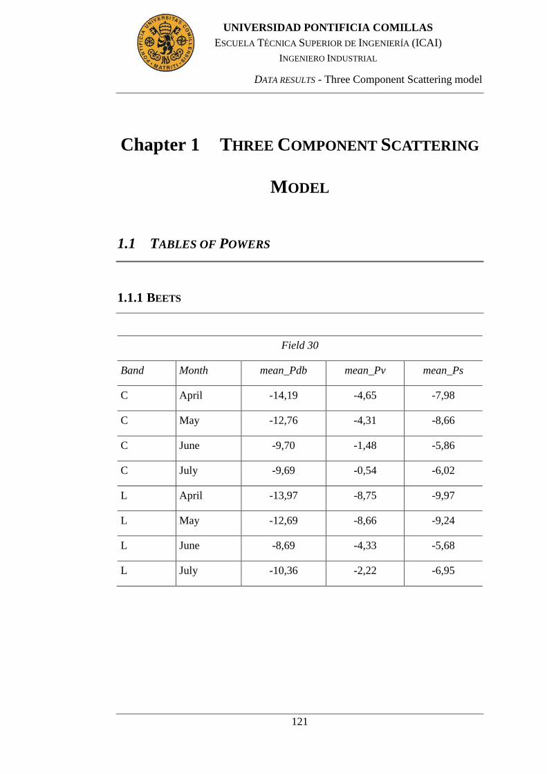
DATA RESULTS - Three Component Scattering model
121
UNIVERSIDAD PONTIFICIA COMILLAS
ESCUELA TÉCNICA SUPERIOR DE INGENIERÍA (ICAI)
INGENIERO INDUSTRIAL
Chapter 1 THREE COMPONENT SCATTERING
MODEL
1.1 TABLES OF POWERS
1.1.1 BEETS
Field 30
Band Month mean_Pdb mean_Pv mean_Ps
C April -14,19 -4,65 -7,98
C May -12,76 -4,31 -8,66
C June -9,70 -1,48 -5,86
C July -9,69 -0,54 -6,02
L April -13,97 -8,75 -9,97
L May -12,69 -8,66 -9,24
L June -8,69 -4,33 -5,68
L July -10,36 -2,22 -6,95
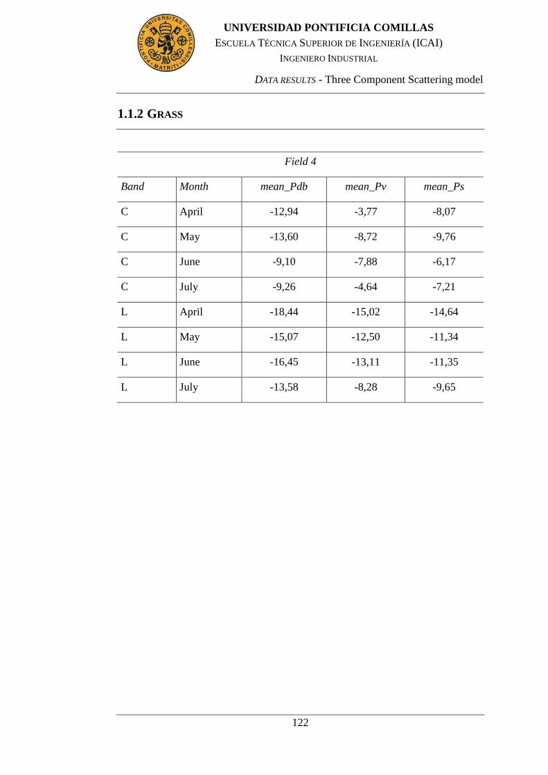
DATA RESULTS - Three Component Scattering model
122
UNIVERSIDAD PONTIFICIA COMILLAS
ESCUELA TÉCNICA SUPERIOR DE INGENIERÍA (ICAI)
INGENIERO INDUSTRIAL
1.1.2 GRASS
Field 4
Band Month mean_Pdb mean_Pv mean_Ps
C April -12,94 -3,77 -8,07
C May -13,60 -8,72 -9,76
C June -9,10 -7,88 -6,17
C July -9,26 -4,64 -7,21
L April -18,44 -15,02 -14,64
L May -15,07 -12,50 -11,34
L June -16,45 -13,11 -11,35
L July -13,58 -8,28 -9,65
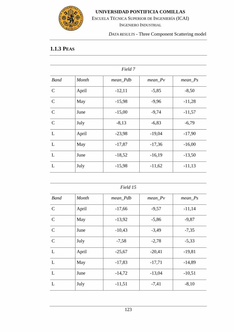
DATA RESULTS - Three Component Scattering model
123
UNIVERSIDAD PONTIFICIA COMILLAS
ESCUELA TÉCNICA SUPERIOR DE INGENIERÍA (ICAI)
INGENIERO INDUSTRIAL
1.1.3 PEAS
Field 7
Band Month mean_Pdb mean_Pv mean_Ps
C April -12,11 -5,85 -8,50
C May -15,98 -9,96 -11,28
C June -15,00 -9,74 -11,57
C July -8,13 -6,83 -6,79
L April -23,98 -19,04 -17,90
L May -17,87 -17,36 -16,00
L June -18,52 -16,19 -13,50
L July -15,98 -11,62 -11,13
Field 15
Band Month mean_Pdb mean_Pv mean_Ps
C April -17,66 -9,57 -11,14
C May -13,92 -5,86 -9,87
C June -10,43 -3,49 -7,35
C July -7,58 -2,78 -5,33
L April -25,67 -20,41 -19,81
L May -17,83 -17,71 -14,89
L June -14,72 -13,04 -10,51
L July -11,51 -7,41 -8,10
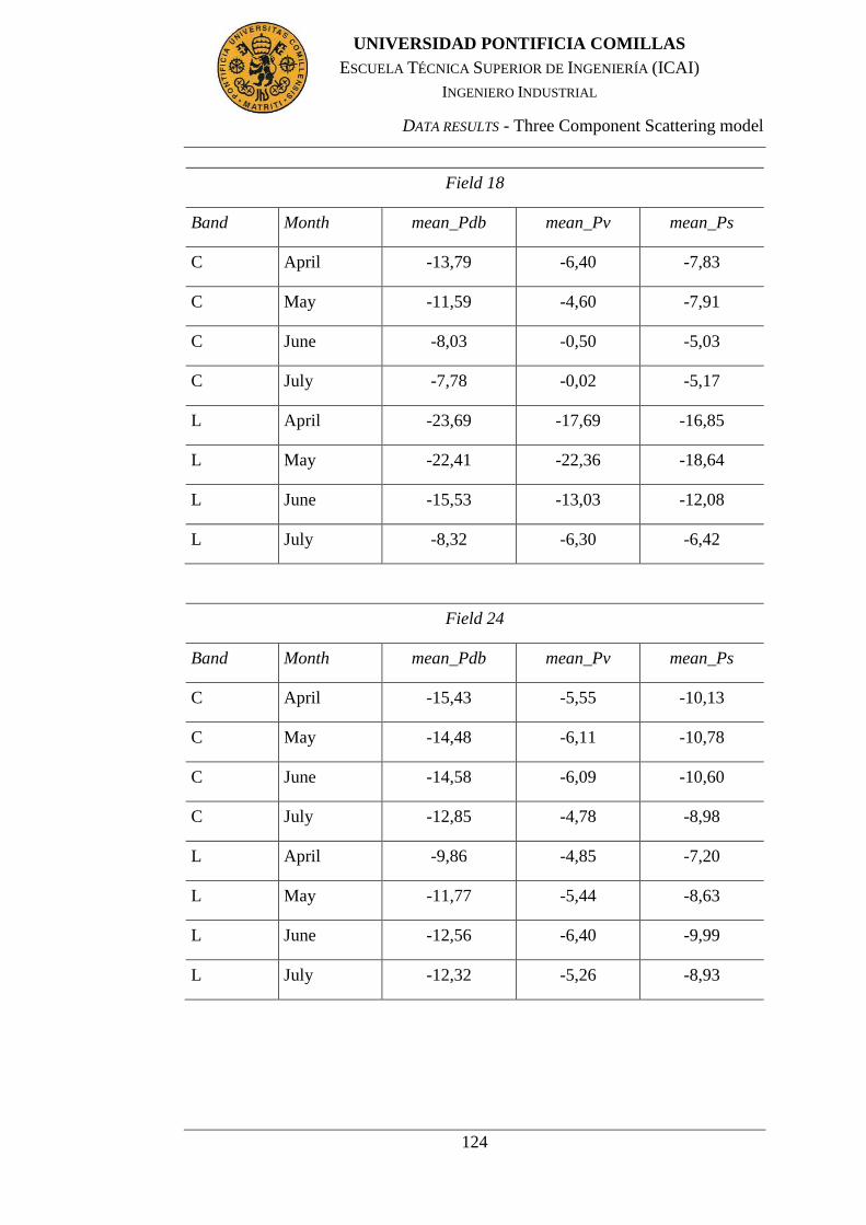
DATA RESULTS - Three Component Scattering model
124
UNIVERSIDAD PONTIFICIA COMILLAS
ESCUELA TÉCNICA SUPERIOR DE INGENIERÍA (ICAI)
INGENIERO INDUSTRIAL
Field 18
Band Month mean_Pdb mean_Pv mean_Ps
C April -13,79 -6,40 -7,83
C May -11,59 -4,60 -7,91
C June -8,03 -0,50 -5,03
C July -7,78 -0,02 -5,17
L April -23,69 -17,69 -16,85
L May -22,41 -22,36 -18,64
L June -15,53 -13,03 -12,08
L July -8,32 -6,30 -6,42
Field 24
Band Month mean_Pdb mean_Pv mean_Ps
C April -15,43 -5,55 -10,13
C May -14,48 -6,11 -10,78
C June -14,58 -6,09 -10,60
C July -12,85 -4,78 -8,98
L April -9,86 -4,85 -7,20
L May -11,77 -5,44 -8,63
L June -12,56 -6,40 -9,99
L July -12,32 -5,26 -8,93
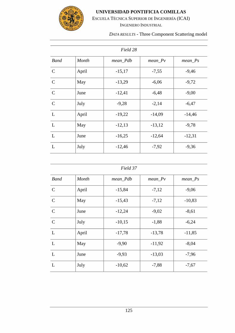
DATA RESULTS - Three Component Scattering model
125
UNIVERSIDAD PONTIFICIA COMILLAS
ESCUELA TÉCNICA SUPERIOR DE INGENIERÍA (ICAI)
INGENIERO INDUSTRIAL
Field 28
Band Month mean_Pdb mean_Pv mean_Ps
C April -15,17 -7,55 -9,46
C May -13,29 -6,06 -9,72
C June -12,41 -6,48 -9,00
C July -9,28 -2,14 -6,47
L April -19,22 -14,09 -14,46
L May -12,13 -13,12 -9,78
L June -16,25 -12,64 -12,31
L July -12,46 -7,92 -9,36
Field 37
Band Month mean_Pdb mean_Pv mean_Ps
C April -15,84 -7,12 -9,06
C May -15,43 -7,12 -10,83
C June -12,24 -9,02 -8,61
C July -10,15 -1,88 -6,24
L April -17,78 -13,78 -11,85
L May -9,90 -11,92 -8,04
L June -9,93 -13,03 -7,96
L July -10,62 -7,88 -7,67

DATA RESULTS - Three Component Scattering model
126
UNIVERSIDAD PONTIFICIA COMILLAS
ESCUELA TÉCNICA SUPERIOR DE INGENIERÍA (ICAI)
INGENIERO INDUSTRIAL
1.1.4 RYE
Field 1
Band Month mean_Pdb mean_Pv mean_Ps
C April -15,53 -5,60 -9,58
C May -14,54 -6,18 -10,82
C June -13,54 -4,32 -9,33
C July -9,58 -2,25 -5,83
L April -9,44 -6,32 -7,60
L May -4,61 -7,95 -3,09
L June -7,35 -7,49 -4,76
L July -10,50 -4,63 -6,66
Field 8
Band Month mean_Pdb mean_Pv mean_Ps
C April -12,14 -3,72 -8,31
C May -14,23 -8,80 -10,44
C June -6,55 -6,64 -4,75
C July -8,63 -3,71 -7,03
L April -21,98 -17,51 -16,32
L May -18,96 -14,74 -13,00
L June -19,03 -15,82 -12,39
L July -15,21 -9,57 -11,44

DATA RESULTS - Three Component Scattering model
127
UNIVERSIDAD PONTIFICIA COMILLAS
ESCUELA TÉCNICA SUPERIOR DE INGENIERÍA (ICAI)
INGENIERO INDUSTRIAL
Field 12
Band Month mean_Pdb mean_Pv mean_Ps
C April -14,08 -4,38 -8,45
C May -13,01 -5,66 -8,76
C June -9,86 -3,38 -6,73
C July -9,85 -2,47 -6,74
L April -13,12 -8,33 -9,59
L May -12,10 -6,93 -8,58
L June -12,96 -6,72 -9,16
L July -10,38 -5,17 -7,23
Field 23
Band Month mean_Pdb mean_Pv mean_Ps
C April -15,68 -8,38 -9,10
C May -13,79 -5,42 -8,95
C June -12,84 -6,71 -8,96
C July -8,29 0,02 -5,22
L April -22,38 -15,97 -15,68
L May -12,22 -14,29 -10,20
L June -15,77 -12,72 -12,14
L July -12,26 -6,20 -9,41

DATA RESULTS - Three Component Scattering model
128
UNIVERSIDAD PONTIFICIA COMILLAS
ESCUELA TÉCNICA SUPERIOR DE INGENIERÍA (ICAI)
INGENIERO INDUSTRIAL
1.1.5 SPRING BARLEY
Field 6
Band Month mean_Pdb mean_Pv mean_Ps
C April -13,46 -5,16 -7,96
C May -13,37 -5,55 -8,43
C June -13,23 -5,95 -8,80
C July -8,96 -1,93 -6,06
L April -15,59 -10,05 -11,24
L May -17,08 -11,74 -13,43
L June -13,53 -9,97 -10,22
L July -11,21 -5,19 -8,10
Field 13
Band Month mean_Pdb mean_Pv mean_Ps
C April -14,18 -5,25 -8,50
C May -14,07 -6,28 -9,68
C June -10,24 -3,09 -7,26
C July -7,95 -2,58 -5,50
L April -13,32 -10,06 -8,60
L May -11,25 -9,95 -8,01
L June -11,78 -8,83 -8,53
L July -8,42 -6,30 -5,62

DATA RESULTS - Three Component Scattering model
129
UNIVERSIDAD PONTIFICIA COMILLAS
ESCUELA TÉCNICA SUPERIOR DE INGENIERÍA (ICAI)
INGENIERO INDUSTRIAL
Field 14
Band Month mean_Pdb mean_Pv mean_Ps
C April -17,27 -6,83 -12,08
C May -16,23 -6,02 -11,30
C June -10,94 -1,70 -7,99
C July -9,61 -4,18 -5,93
L April -12,01 -9,45 -10,54
L May -4,49 -11,07 -3,58
L June -16,33 -8,86 -13,62
L July -11,54 -8,74 -8,19
Field 29
Band Month mean_Pdb mean_Pv mean_Ps
C April -14,93 -5,37 -8,74
C May -15,73 -7,94 -11,55
C June -15,13 -7,68 -10,67
C July -11,71 -3,32 -8,39
L April -13,64 -7,01 -8,79
L May -16,55 -9,88 -11,29
L June -17,57 -10,06 -11,45
L July -13,27 -5,85 -8,75

DATA RESULTS - Three Component Scattering model
130
UNIVERSIDAD PONTIFICIA COMILLAS
ESCUELA TÉCNICA SUPERIOR DE INGENIERÍA (ICAI)
INGENIERO INDUSTRIAL
Field 31
Band Month mean_Pdb mean_Pv mean_Ps
C April -14,54 -7,12 -8,25
C May -13,06 -5,14 -8,98
C June -10,39 -1,60 -6,01
C July -9,72 -1,40 -6,21
L April -18,31 -13,01 -14,21
L May -16,13 -12,29 -12,55
L June -10,40 -5,16 -7,17
L July -11,04 -4,08 -7,80
Field 34
Band Month mean_Pdb mean_Pv mean_Ps
C April -18,19 -10,63 -9,60
C May -16,29 -7,67 -10,91
C June -13,69 -7,31 -9,92
C July -6,90 -0,67 -4,31
L April -27,65 -21,74 -19,61
L May -16,27 -19,31 -14,82
L June -16,42 -14,15 -13,06
L July -9,84 -7,33 -8,22
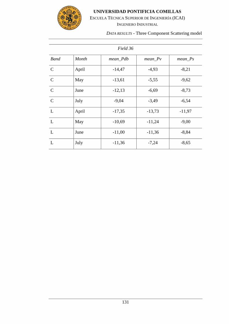
DATA RESULTS - Three Component Scattering model
131
UNIVERSIDAD PONTIFICIA COMILLAS
ESCUELA TÉCNICA SUPERIOR DE INGENIERÍA (ICAI)
INGENIERO INDUSTRIAL
Field 36
Band Month mean_Pdb mean_Pv mean_Ps
C April -14,47 -4,93 -8,21
C May -13,61 -5,55 -9,62
C June -12,13 -6,69 -8,73
C July -9,04 -3,49 -6,54
L April -17,35 -13,73 -11,97
L May -10,69 -11,24 -9,00
L June -11,00 -11,36 -8,84
L July -11,36 -7,24 -8,65

DATA RESULTS - Three Component Scattering model
132
UNIVERSIDAD PONTIFICIA COMILLAS
ESCUELA TÉCNICA SUPERIOR DE INGENIERÍA (ICAI)
INGENIERO INDUSTRIAL
1.1.6 SPRING OATS
Field 9
Band Month mean_Pdb mean_Pv mean_Ps
C April -15,56 -7,69 -10,42
C May -14,87 -7,53 -10,44
C June -10,31 -6,76 -6,58
C July -8,30 -3,62 -6,45
L April -27,29 -21,71 -20,20
L May -10,05 -17,65 -7,49
L June -19,41 -16,26 -13,74
L July -13,68 -10,44 -10,41
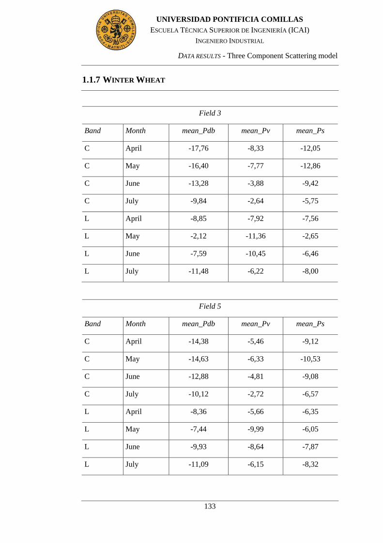
DATA RESULTS - Three Component Scattering model
133
UNIVERSIDAD PONTIFICIA COMILLAS
ESCUELA TÉCNICA SUPERIOR DE INGENIERÍA (ICAI)
INGENIERO INDUSTRIAL
1.1.7 WINTER WHEAT
Field 3
Band Month mean_Pdb mean_Pv mean_Ps
C April -17,76 -8,33 -12,05
C May -16,40 -7,77 -12,86
C June -13,28 -3,88 -9,42
C July -9,84 -2,64 -5,75
L April -8,85 -7,92 -7,56
L May -2,12 -11,36 -2,65
L June -7,59 -10,45 -6,46
L July -11,48 -6,22 -8,00
Field 5
Band Month mean_Pdb mean_Pv mean_Ps
C April -14,38 -5,46 -9,12
C May -14,63 -6,33 -10,53
C June -12,88 -4,81 -9,08
C July -10,12 -2,72 -6,57
L April -8,36 -5,66 -6,35
L May -7,44 -9,99 -6,05
L June -9,93 -8,64 -7,87
L July -11,09 -6,15 -8,32
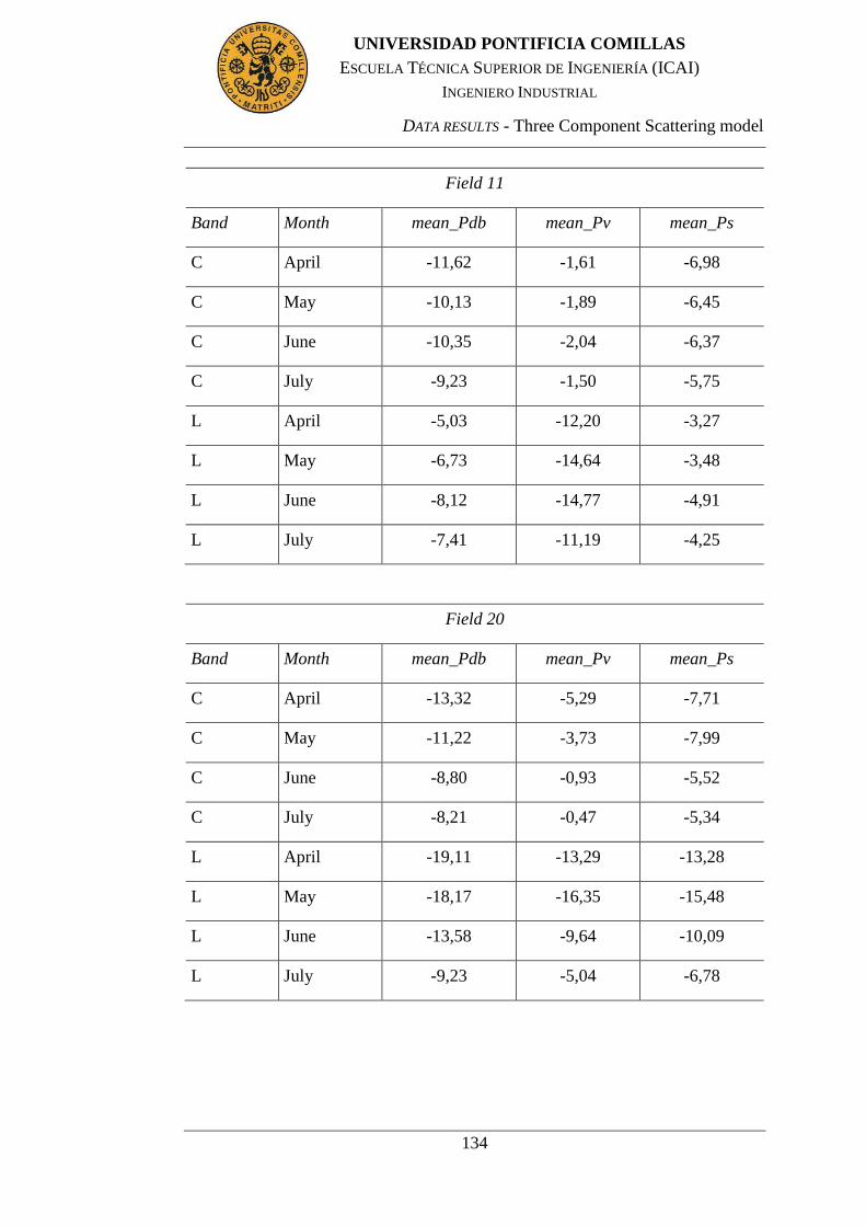
DATA RESULTS - Three Component Scattering model
134
UNIVERSIDAD PONTIFICIA COMILLAS
ESCUELA TÉCNICA SUPERIOR DE INGENIERÍA (ICAI)
INGENIERO INDUSTRIAL
Field 11
Band Month mean_Pdb mean_Pv mean_Ps
C April -11,62 -1,61 -6,98
C May -10,13 -1,89 -6,45
C June -10,35 -2,04 -6,37
C July -9,23 -1,50 -5,75
L April -5,03 -12,20 -3,27
L May -6,73 -14,64 -3,48
L June -8,12 -14,77 -4,91
L July -7,41 -11,19 -4,25
Field 20
Band Month mean_Pdb mean_Pv mean_Ps
C April -13,32 -5,29 -7,71
C May -11,22 -3,73 -7,99
C June -8,80 -0,93 -5,52
C July -8,21 -0,47 -5,34
L April -19,11 -13,29 -13,28
L May -18,17 -16,35 -15,48
L June -13,58 -9,64 -10,09
L July -9,23 -5,04 -6,78
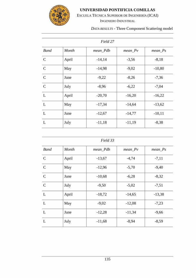
DATA RESULTS - Three Component Scattering model
135
UNIVERSIDAD PONTIFICIA COMILLAS
ESCUELA TÉCNICA SUPERIOR DE INGENIERÍA (ICAI)
INGENIERO INDUSTRIAL
Field 27
Band Month mean_Pdb mean_Pv mean_Ps
C April -14,14 -3,56 -8,18
C May -14,98 -9,02 -10,80
C June -9,22 -8,26 -7,36
C July -8,96 -6,22 -7,04
L April -20,70 -16,20 -16,22
L May -17,34 -14,64 -13,62
L June -12,67 -14,77 -10,11
L July -11,18 -11,19 -8,38
Field 33
Band Month mean_Pdb mean_Pv mean_Ps
C April -13,67 -4,74 -7,11
C May -12,96 -5,70 -9,40
C June -10,68 -6,28 -8,32
C July -9,50 -5,02 -7,51
L April -18,72 -14,65 -13,38
L May -9,02 -12,08 -7,23
L June -12,28 -11,34 -9,66
L July -11,68 -8,94 -8,59
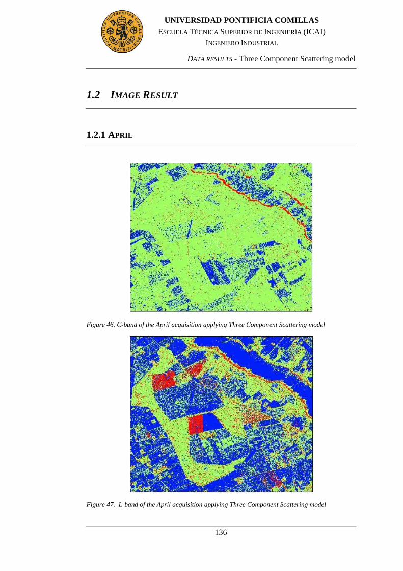
DATA RESULTS - Three Component Scattering model
136
UNIVERSIDAD PONTIFICIA COMILLAS
ESCUELA TÉCNICA SUPERIOR DE INGENIERÍA (ICAI)
INGENIERO INDUSTRIAL
1.2 IMAGE RESULT
1.2.1 APRIL
Figure 46. C-band of the April acquisition applying Three Component Scattering model
Figure 47. L-band of the April acquisition applying Three Component Scattering model
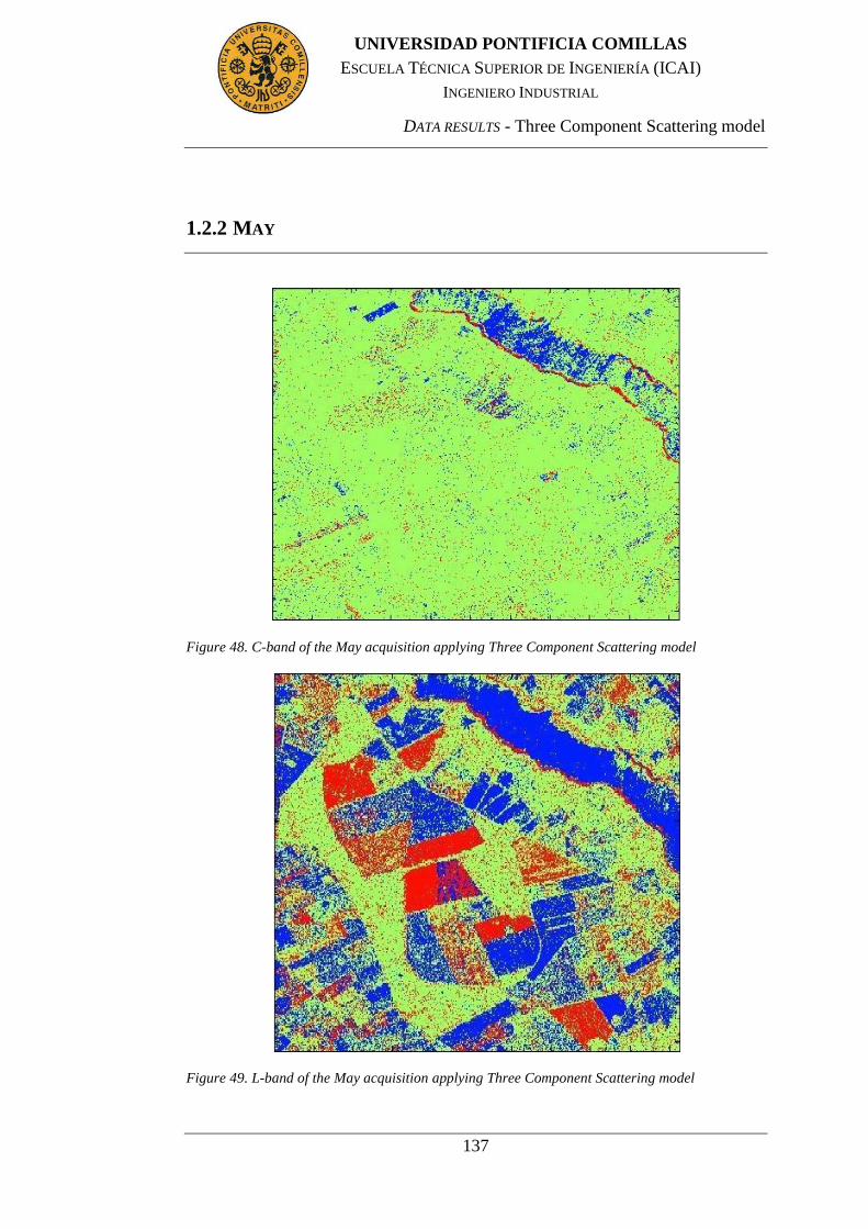
DATA RESULTS - Three Component Scattering model
137
UNIVERSIDAD PONTIFICIA COMILLAS
ESCUELA TÉCNICA SUPERIOR DE INGENIERÍA (ICAI)
INGENIERO INDUSTRIAL
1.2.2 MAY
Figure 48. C-band of the May acquisition applying Three Component Scattering model
Figure 49. L-band of the May acquisition applying Three Component Scattering model
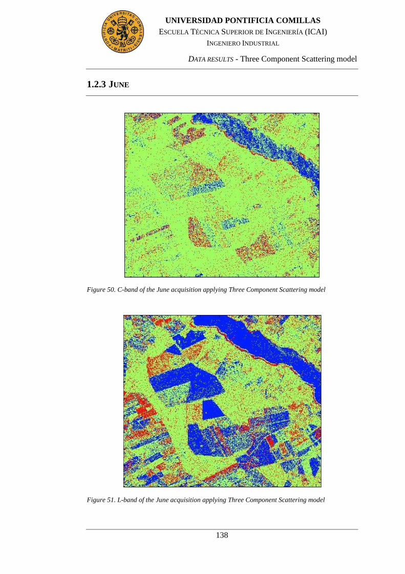
DATA RESULTS - Three Component Scattering model
138
UNIVERSIDAD PONTIFICIA COMILLAS
ESCUELA TÉCNICA SUPERIOR DE INGENIERÍA (ICAI)
INGENIERO INDUSTRIAL
1.2.3 JUNE
Figure 50. C-band of the June acquisition applying Three Component Scattering model
Figure 51. L-band of the June acquisition applying Three Component Scattering model
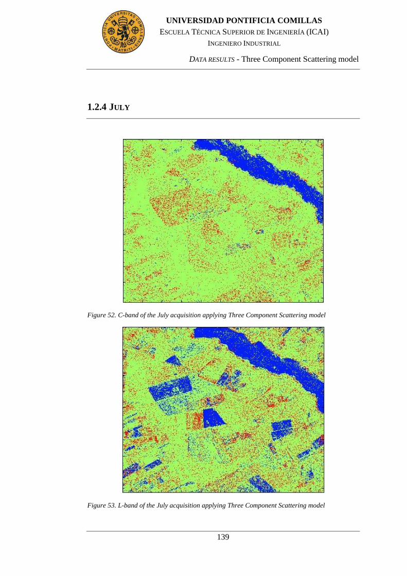
DATA RESULTS - Three Component Scattering model
139
UNIVERSIDAD PONTIFICIA COMILLAS
ESCUELA TÉCNICA SUPERIOR DE INGENIERÍA (ICAI)
INGENIERO INDUSTRIAL
1.2.4 JULY
Figure 52. C-band of the July acquisition applying Three Component Scattering model
Figure 53. L-band of the July acquisition applying Three Component Scattering model
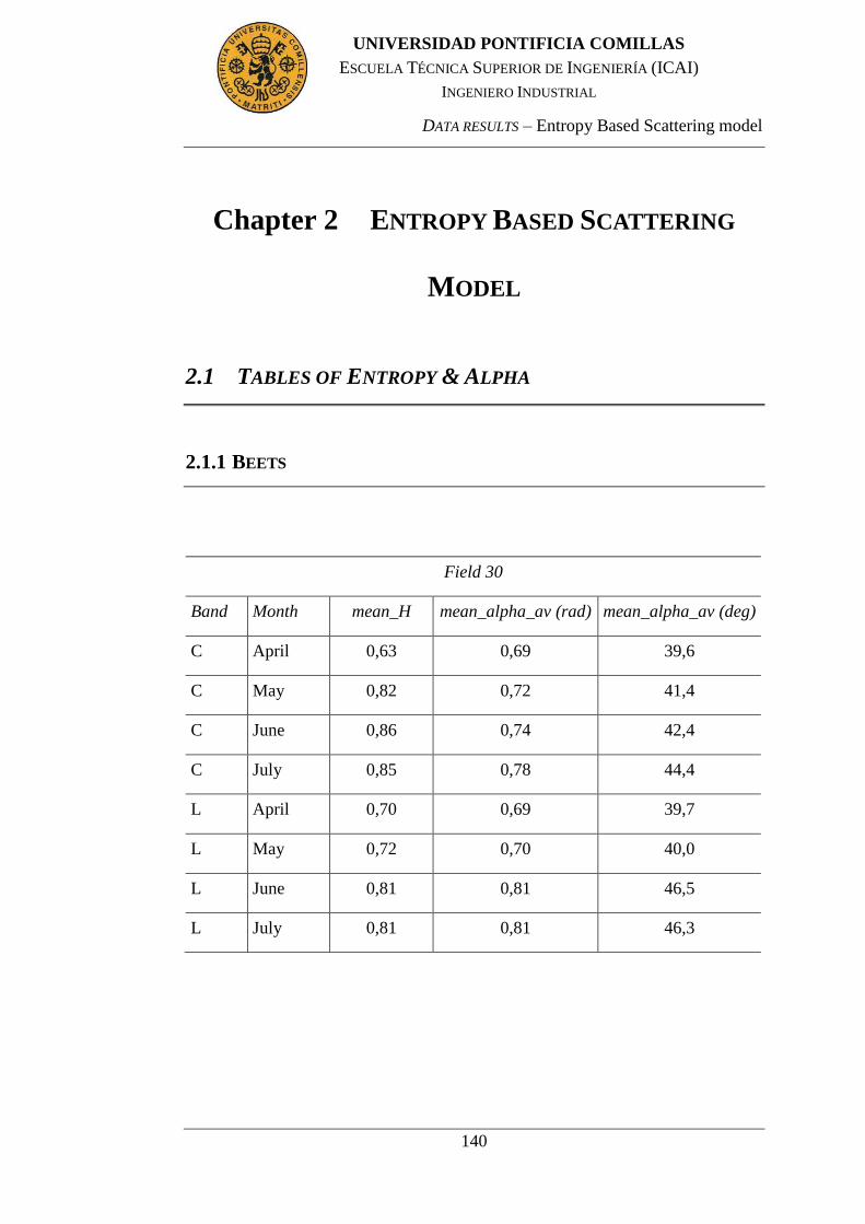
DATA RESULTS – Entropy Based Scattering model
140
UNIVERSIDAD PONTIFICIA COMILLAS
ESCUELA TÉCNICA SUPERIOR DE INGENIERÍA (ICAI)
INGENIERO INDUSTRIAL
Chapter 2 ENTROPY BASED SCATTERING
MODEL
2.1 TABLES OF ENTROPY & ALPHA
2.1.1 BEETS
Field 30
Band Month mean_H mean_alpha_av (rad) mean_alpha_av (deg)
C April 0,63 0,69 39,6
C May 0,82 0,72 41,4
C June 0,86 0,74 42,4
C July 0,85 0,78 44,4
L April 0,70 0,69 39,7
L May 0,72 0,70 40,0
L June 0,81 0,81 46,5
L July 0,81 0,81 46,3

DATA RESULTS – Entropy Based Scattering model
141
UNIVERSIDAD PONTIFICIA COMILLAS
ESCUELA TÉCNICA SUPERIOR DE INGENIERÍA (ICAI)
INGENIERO INDUSTRIAL
2.1.2 GRASS
Field 4
Band Month mean_H mean_alpha_av (rad) mean_alpha_av (deg)
C April 0,74 0,72 41,4
C May 0,76 0,76 43,8
C June 0,79 0,78 44,9
C July 0,85 0,83 47,7
L April 0,60 0,71 40,7
L May 0,61 0,65 37,0
L June 0,56 0,55 31,7
L July 0,70 0,67 38,5

DATA RESULTS – Entropy Based Scattering model
142
UNIVERSIDAD PONTIFICIA COMILLAS
ESCUELA TÉCNICA SUPERIOR DE INGENIERÍA (ICAI)
INGENIERO INDUSTRIAL
2.1.3 PEAS
Field 7
Band Month mean_H mean_alpha_av (rad) mean_alpha_av (deg)
C April 0,72 0,73 41,9
C May 0,74 0,80 46,0
C June 0,82 0,70 40,2
C July 0,83 0,83 47,6
L April 0,50 0,61 35,0
L May 0,59 0,71 40,8
L June 0,50 0,49 28,2
L July 0,62 0,57 32,5
Field 15
Band Month mean_H mean_alpha_av (rad) mean_alpha_av (deg)
C April 0,52 0,71 40,4
C May 0,80 0,73 41,7
C June 0,87 0,77 44,2
C July 0,84 0,82 46,9
L April 0,58 0,61 34,7
L May 0,64 0,72 41,3
L June 0,63 0,67 38,6
L July 0,67 0,69 39,3

DATA RESULTS – Entropy Based Scattering model
143
UNIVERSIDAD PONTIFICIA COMILLAS
ESCUELA TÉCNICA SUPERIOR DE INGENIERÍA (ICAI)
INGENIERO INDUSTRIAL
Field 18
Band Month mean_H mean_alpha_av (rad) mean_alpha_av (deg)
C April 0,44 0,58 33,2
C May 0,78 0,70 40,3
C June 0,89 0,81 46,1
C July 0,87 0,82 46,8
L April 0,53 0,58 33,1
L May 0,48 0,55 31,4
L June 0,70 0,69 39,4
L July 0,78 0,80 45,8
Field 24
Band Month mean_H mean_alpha_av (rad) mean_alpha_av (deg)
C April 0,69 0,74 42,3
C May 0,82 0,75 43,3
C June 0,83 0,70 40,2
C July 0,81 0,74 42,6
L April 0,77 0,79 45,0
L May 0,84 0,80 45,9
L June 0,83 0,82 47,2
L July 0,82 0,80 46,1

DATA RESULTS – Entropy Based Scattering model
144
UNIVERSIDAD PONTIFICIA COMILLAS
ESCUELA TÉCNICA SUPERIOR DE INGENIERÍA (ICAI)
INGENIERO INDUSTRIAL
Field 28
Band Month mean_H mean_alpha_av (rad) mean_alpha_av (deg)
C April 0,57 0,73 41,6
C May 0,81 0,76 43,3
C June 0,81 0,77 44,0
C July 0,79 0,83 47,3
L April 0,62 0,68 38,7
L May 0,76 0,80 45,6
L June 0,70 0,69 39,7
L July 0,75 0,77 44,3
Field 37
Band Month mean_H mean_alpha_av (rad) mean_alpha_av (deg)
C April 0,57 0,60 34,3
C May 0,76 0,69 39,7
C June 0,77 0,72 41,4
C July 0,78 0,80 45,9
L April 0,49 0,58 33,1
L May 0,80 0,83 47,8
L June 0,77 0,85 48,5
L July 0,79 0,84 48,0
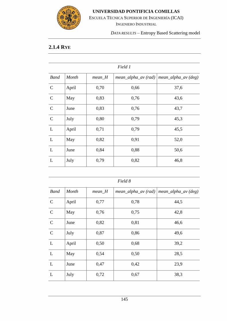
DATA RESULTS – Entropy Based Scattering model
145
UNIVERSIDAD PONTIFICIA COMILLAS
ESCUELA TÉCNICA SUPERIOR DE INGENIERÍA (ICAI)
INGENIERO INDUSTRIAL
2.1.4 RYE
Field 1
Band Month mean_H mean_alpha_av (rad) mean_alpha_av (deg)
C April 0,70 0,66 37,6
C May 0,83 0,76 43,6
C June 0,83 0,76 43,7
C July 0,80 0,79 45,3
L April 0,71 0,79 45,5
L May 0,82 0,91 52,0
L June 0,84 0,88 50,6
L July 0,79 0,82 46,8
Field 8
Band Month mean_H mean_alpha_av (rad) mean_alpha_av (deg)
C April 0,77 0,78 44,5
C May 0,76 0,75 42,8
C June 0,82 0,81 46,6
C July 0,87 0,86 49,6
L April 0,50 0,68 39,2
L May 0,54 0,50 28,5
L June 0,47 0,42 23,9
L July 0,72 0,67 38,3

DATA RESULTS – Entropy Based Scattering model
146
UNIVERSIDAD PONTIFICIA COMILLAS
ESCUELA TÉCNICA SUPERIOR DE INGENIERÍA (ICAI)
INGENIERO INDUSTRIAL
Field 12
Band Month mean_H mean_alpha_av (rad) mean_alpha_av (deg)
C April 0,67 0,70 39,9
C May 0,77 0,73 41,8
C June 0,83 0,78 44,6
C July 0,84 0,79 45,2
L April 0,71 0,74 42,7
L May 0,78 0,77 44,4
L June 0,76 0,76 43,3
L July 0,79 0,80 46,0
Field 23
Band Month mean_H mean_alpha_av (rad) mean_alpha_av (deg)
C April 0,43 0,61 35,0
C May 0,77 0,67 38,2
C June 0,79 0,71 40,6
C July 0,81 0,83 47,3
L April 0,55 0,59 33,8
L May 0,76 0,80 46,0
L June 0,72 0,77 43,9
L July 0,79 0,82 47,0

DATA RESULTS – Entropy Based Scattering model
147
UNIVERSIDAD PONTIFICIA COMILLAS
ESCUELA TÉCNICA SUPERIOR DE INGENIERÍA (ICAI)
INGENIERO INDUSTRIAL
2.1.5 SPRING BARLEY
Field 6
Band Month mean_H mean_alpha_av (rad) mean_alpha_av (deg)
C April 0,61 0,66 37,8
C May 0,74 0,64 36,7
C June 0,79 0,67 38,3
C July 0,82 0,80 45,6
L April 0,68 0,69 39,5
L May 0,77 0,73 41,8
L June 0,77 0,78 44,9
L July 0,80 0,82 46,8
Field 13
Band Month mean_H mean_alpha_av (rad) mean_alpha_av (deg)
C April 0,62 0,66 37,7
C May 0,77 0,72 41,2
C June 0,85 0,79 45,3
C July 0,83 0,81 46,2
L April 0,58 0,68 38,8
L May 0,74 0,77 43,9
L June 0,73 0,77 44,4
L July 0,78 0,83 47,5

DATA RESULTS – Entropy Based Scattering model
148
UNIVERSIDAD PONTIFICIA COMILLAS
ESCUELA TÉCNICA SUPERIOR DE INGENIERÍA (ICAI)
INGENIERO INDUSTRIAL
Field 14
Band Month mean_H mean_alpha_av (rad) mean_alpha_av (deg)
C April 0,74 0,72 41,3
C May 0,81 0,74 42,4
C June 0,89 0,84 48,1
C July 0,80 0,83 47,7
L April 0,68 0,80 45,6
L May 0,88 0,94 54,0
L June 0,84 0,85 48,6
L July 0,83 0,89 51,0
Field 29
Band Month mean_H mean_alpha_av (rad) mean_alpha_av (deg)
C April 0,66 0,61 35,1
C May 0,79 0,70 40,3
C June 0,83 0,66 37,8
C July 0,85 0,77 44,1
L April 0,71 0,66 38,0
L May 0,68 0,59 33,6
L June 0,65 0,59 33,9
L July 0,75 0,75 43,0

DATA RESULTS – Entropy Based Scattering model
149
UNIVERSIDAD PONTIFICIA COMILLAS
ESCUELA TÉCNICA SUPERIOR DE INGENIERÍA (ICAI)
INGENIERO INDUSTRIAL
Field 31
Band Month mean_H mean_alpha_av (rad) mean_alpha_av (deg)
C April 0,59 0,63 36,1
C May 0,81 0,72 41,1
C June 0,84 0,73 41,6
C July 0,83 0,76 43,8
L April 0,69 0,67 38,7
L May 0,71 0,73 41,7
L June 0,78 0,77 44,3
L July 0,78 0,78 44,7
Field 34
Band Month mean_H mean_alpha_av (rad) mean_alpha_av (deg)
C April 0,44 0,48 27,7
C May 0,76 0,64 36,5
C June 0,80 0,73 42,0
C July 0,78 0,84 48,1
L April 0,42 0,47 27,2
L May 0,73 0,74 42,3
L June 0,72 0,78 44,6
L July 0,83 0,86 49,1

DATA RESULTS – Entropy Based Scattering model
150
UNIVERSIDAD PONTIFICIA COMILLAS
ESCUELA TÉCNICA SUPERIOR DE INGENIERÍA (ICAI)
INGENIERO INDUSTRIAL
Field 36
Band Month mean_H mean_alpha_av (rad) mean_alpha_av (deg)
C April 0,66 0,62 35,4
C May 0,81 0,74 42,7
C June 0,83 0,74 42,3
C July 0,84 0,81 46,1
L April 0,51 0,57 32,9
L May 0,82 0,83 47,6
L June 0,74 0,78 44,8
L July 0,78 0,78 44,7
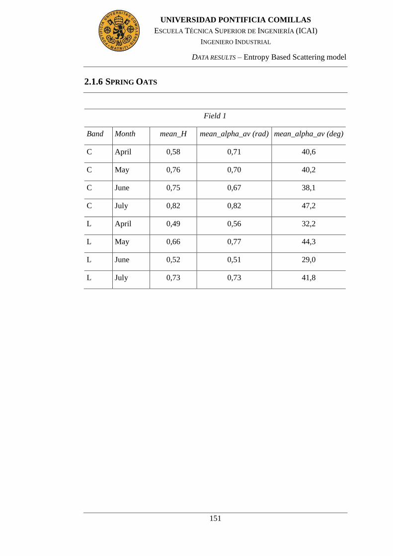
DATA RESULTS – Entropy Based Scattering model
151
UNIVERSIDAD PONTIFICIA COMILLAS
ESCUELA TÉCNICA SUPERIOR DE INGENIERÍA (ICAI)
INGENIERO INDUSTRIAL
2.1.6 SPRING OATS
Field 1
Band Month mean_H mean_alpha_av (rad) mean_alpha_av (deg)
C April 0,58 0,71 40,6
C May 0,76 0,70 40,2
C June 0,75 0,67 38,1
C July 0,82 0,82 47,2
L April 0,49 0,56 32,2
L May 0,66 0,77 44,3
L June 0,52 0,51 29,0
L July 0,73 0,73 41,8
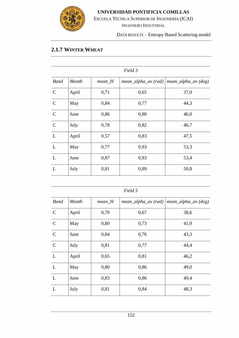
DATA RESULTS – Entropy Based Scattering model
152
UNIVERSIDAD PONTIFICIA COMILLAS
ESCUELA TÉCNICA SUPERIOR DE INGENIERÍA (ICAI)
INGENIERO INDUSTRIAL
2.1.7 WINTER WHEAT
Field 3
Band Month mean_H mean_alpha_av (rad) mean_alpha_av (deg)
C April 0,71 0,65 37,0
C May 0,84 0,77 44,3
C June 0,86 0,80 46,0
C July 0,78 0,82 46,7
L April 0,57 0,83 47,5
L May 0,77 0,93 53,3
L June 0,87 0,93 53,4
L July 0,81 0,89 50,8
Field 5
Band Month mean_H mean_alpha_av (rad) mean_alpha_av (deg)
C April 0,70 0,67 38,6
C May 0,80 0,73 41,9
C June 0,84 0,76 43,3
C July 0,81 0,77 44,4
L April 0,65 0,81 46,2
L May 0,80 0,86 49,0
L June 0,83 0,86 49,4
L July 0,81 0,84 48,3

DATA RESULTS – Entropy Based Scattering model
153
UNIVERSIDAD PONTIFICIA COMILLAS
ESCUELA TÉCNICA SUPERIOR DE INGENIERÍA (ICAI)
INGENIERO INDUSTRIAL
Field 11
Band Month mean_H mean_alpha_av (rad) mean_alpha_av (deg)
C April 0,76 0,77 43,9
C May 0,83 0,76 43,8
C June 0,84 0,74 42,3
C July 0,84 0,77 44,4
L April 0,81 0,84 48,0
L May 0,84 0,84 48,4
L June 0,82 0,82 47,2
L July 0,83 0,83 47,6
Field 20
Band Month mean_H mean_alpha_av (rad) mean_alpha_av (deg)
C April 0,52 0,65 37,1
C May 0,84 0,77 44,3
C June 0,88 0,78 44,9
C July 0,86 0,80 45,9
L April 0,58 0,63 36,2
L May 0,65 0,73 41,8
L June 0,73 0,74 42,1
L July 0,80 0,80 46,0

DATA RESULTS – Entropy Based Scattering model
154
UNIVERSIDAD PONTIFICIA COMILLAS
ESCUELA TÉCNICA SUPERIOR DE INGENIERÍA (ICAI)
INGENIERO INDUSTRIAL
Field 27
Band Month mean_H mean_alpha_av (rad) mean_alpha_av (deg)
C April 0,67 0,74 42,4
C May 0,74 0,74 42,6
C June 0,81 0,78 44,6
C July 0,82 0,80 45,9
L April 0,61 0,67 38,3
L May 0,65 0,65 37,3
L June 0,65 0,72 41,2
L July 0,64 0,71 40,5
Field 33
Band Month mean_H mean_alpha_av (rad) mean_alpha_av (deg)
C April 0,61 0,57 32,5
C May 0,80 0,77 44,0
C June 0,85 0,80 46,0
C July 0,84 0,82 46,8
L April 0,53 0,54 30,9
L May 0,80 0,84 48,4
L June 0,75 0,76 43,8
L July 0,74 0,74 42,6
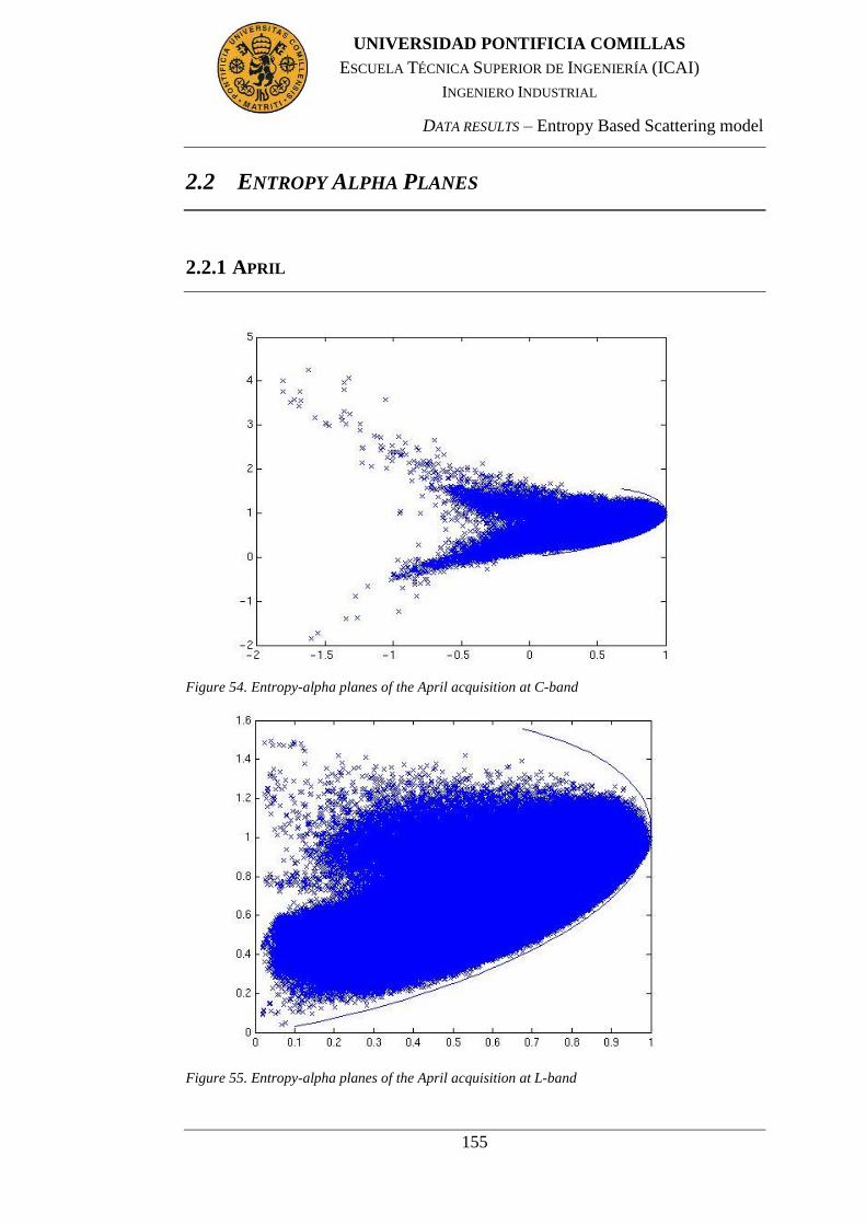
DATA RESULTS – Entropy Based Scattering model
155
UNIVERSIDAD PONTIFICIA COMILLAS
ESCUELA TÉCNICA SUPERIOR DE INGENIERÍA (ICAI)
INGENIERO INDUSTRIAL
2.2 ENTROPY ALPHA PLANES
2.2.1 APRIL
Figure 54. Entropy-alpha planes of the April acquisition at C-band
Figure 55. Entropy-alpha planes of the April acquisition at L-band
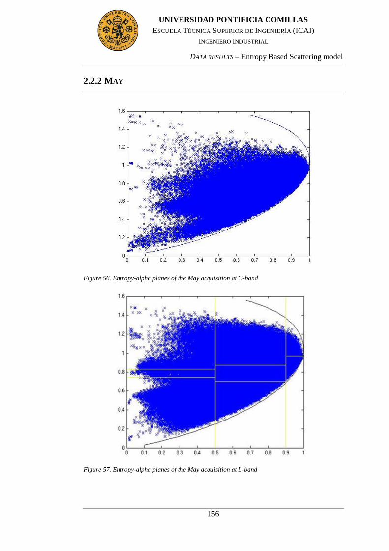
DATA RESULTS – Entropy Based Scattering model
156
UNIVERSIDAD PONTIFICIA COMILLAS
ESCUELA TÉCNICA SUPERIOR DE INGENIERÍA (ICAI)
INGENIERO INDUSTRIAL
2.2.2 MAY
Figure 56. Entropy-alpha planes of the May acquisition at C-band
Figure 57. Entropy-alpha planes of the May acquisition at L-band
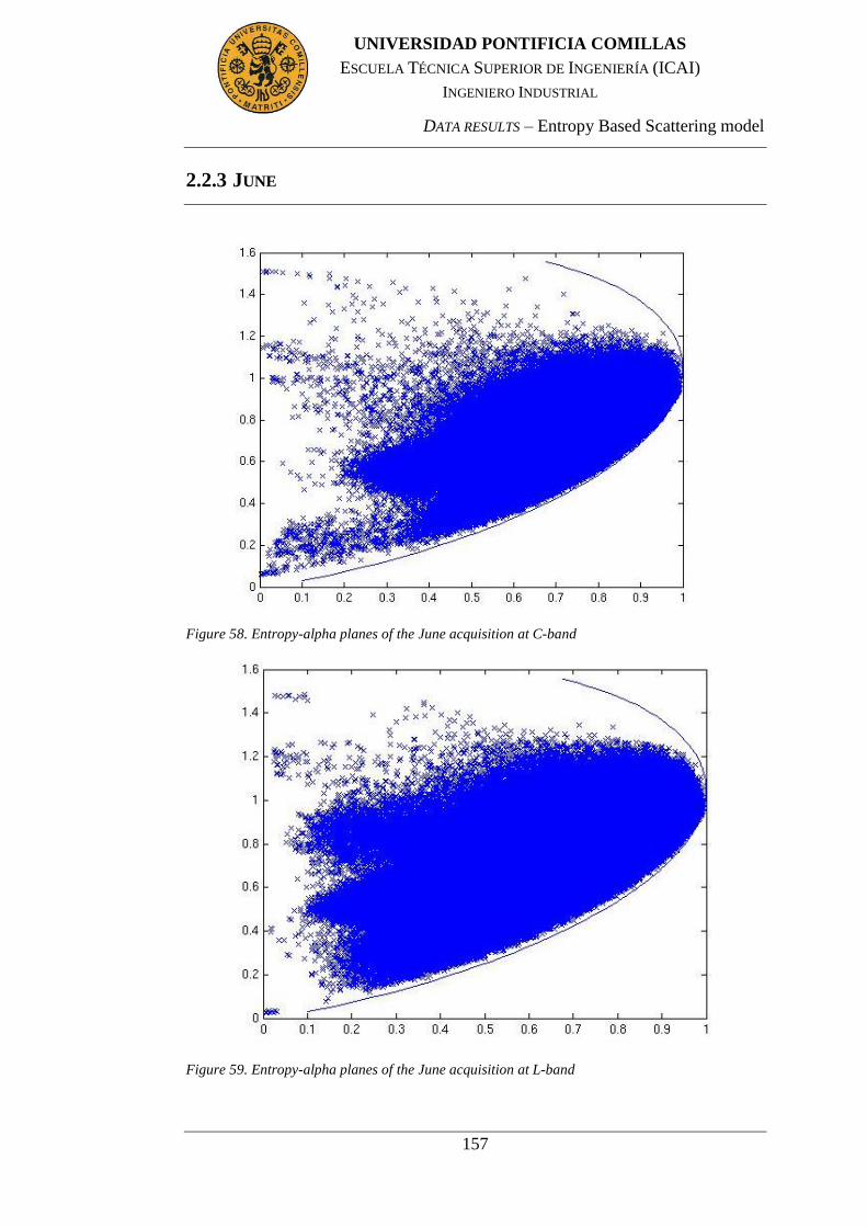
DATA RESULTS – Entropy Based Scattering model
157
UNIVERSIDAD PONTIFICIA COMILLAS
ESCUELA TÉCNICA SUPERIOR DE INGENIERÍA (ICAI)
INGENIERO INDUSTRIAL
2.2.3 JUNE
Figure 58. Entropy-alpha planes of the June acquisition at C-band
Figure 59. Entropy-alpha planes of the June acquisition at L-band
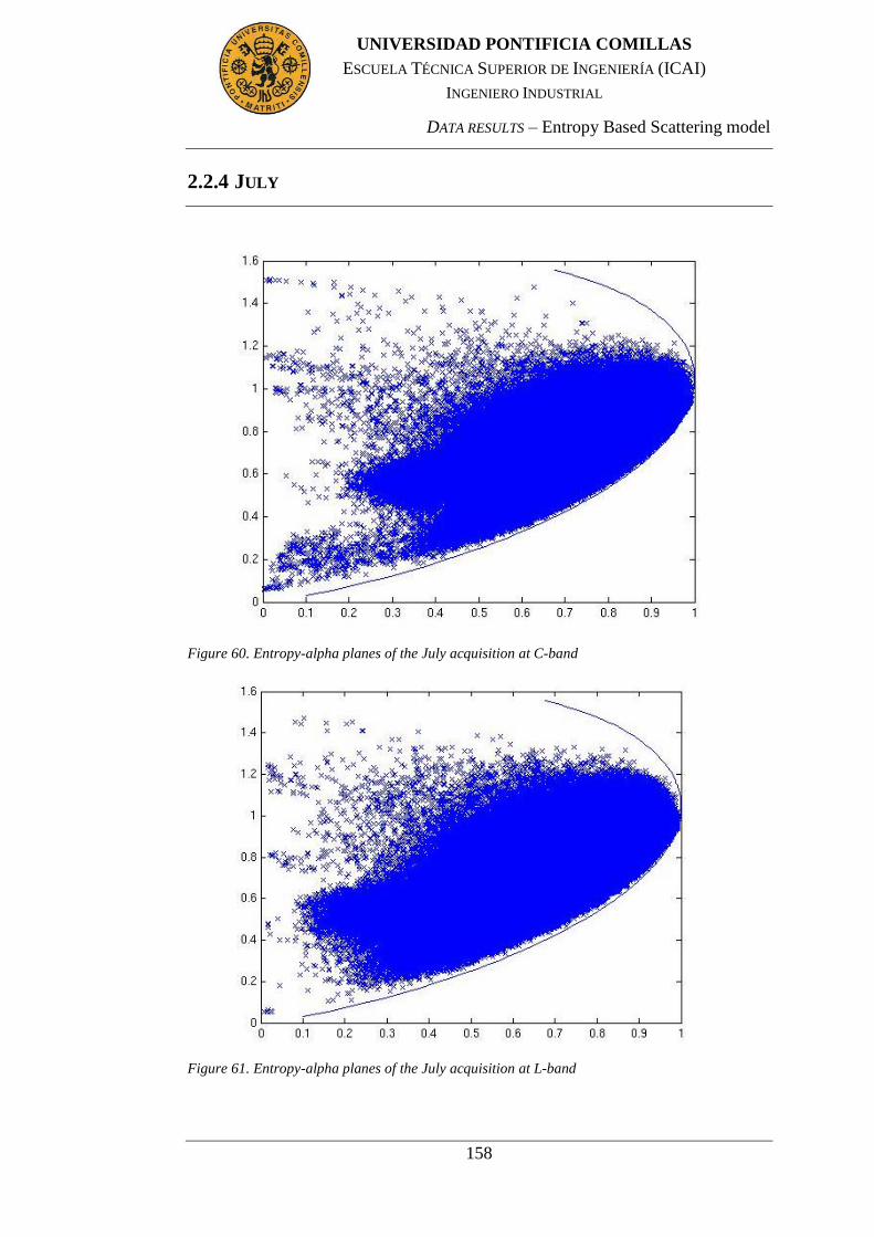
DATA RESULTS – Entropy Based Scattering model
158
UNIVERSIDAD PONTIFICIA COMILLAS
ESCUELA TÉCNICA SUPERIOR DE INGENIERÍA (ICAI)
INGENIERO INDUSTRIAL
2.2.4 JULY
Figure 60. Entropy-alpha planes of the July acquisition at C-band
Figure 61. Entropy-alpha planes of the July acquisition at L-band
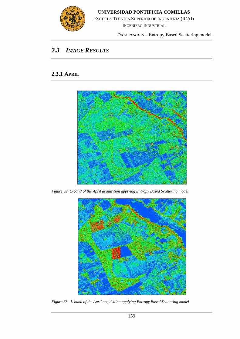
DATA RESULTS – Entropy Based Scattering model
159
UNIVERSIDAD PONTIFICIA COMILLAS
ESCUELA TÉCNICA SUPERIOR DE INGENIERÍA (ICAI)
INGENIERO INDUSTRIAL
2.3 IMAGE RESULTS
2.3.1 APRIL
Figure 62. C-band of the April acquisition applying Entropy Based Scattering model
Figure 63. L-band of the April acquisition applying Entropy Based Scattering model
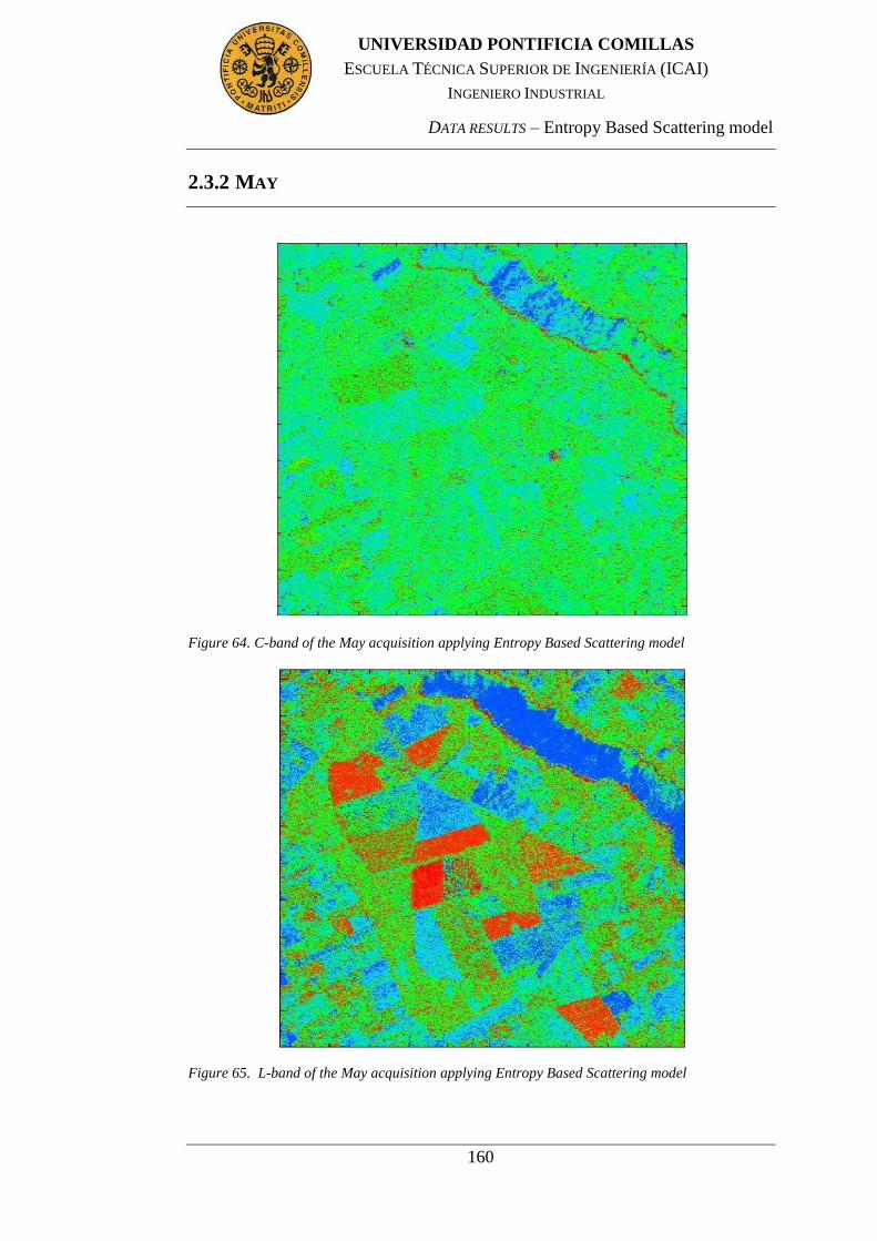
DATA RESULTS – Entropy Based Scattering model
160
UNIVERSIDAD PONTIFICIA COMILLAS
ESCUELA TÉCNICA SUPERIOR DE INGENIERÍA (ICAI)
INGENIERO INDUSTRIAL
2.3.2 MAY
Figure 64. C-band of the May acquisition applying Entropy Based Scattering model
Figure 65. L-band of the May acquisition applying Entropy Based Scattering model
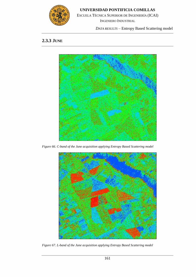
DATA RESULTS – Entropy Based Scattering model
161
UNIVERSIDAD PONTIFICIA COMILLAS
ESCUELA TÉCNICA SUPERIOR DE INGENIERÍA (ICAI)
INGENIERO INDUSTRIAL
2.3.3 JUNE
Figure 66. C-band of the June acquisition applying Entropy Based Scattering model
Figure 67. L-band of the June acquisition applying Entropy Based Scattering model
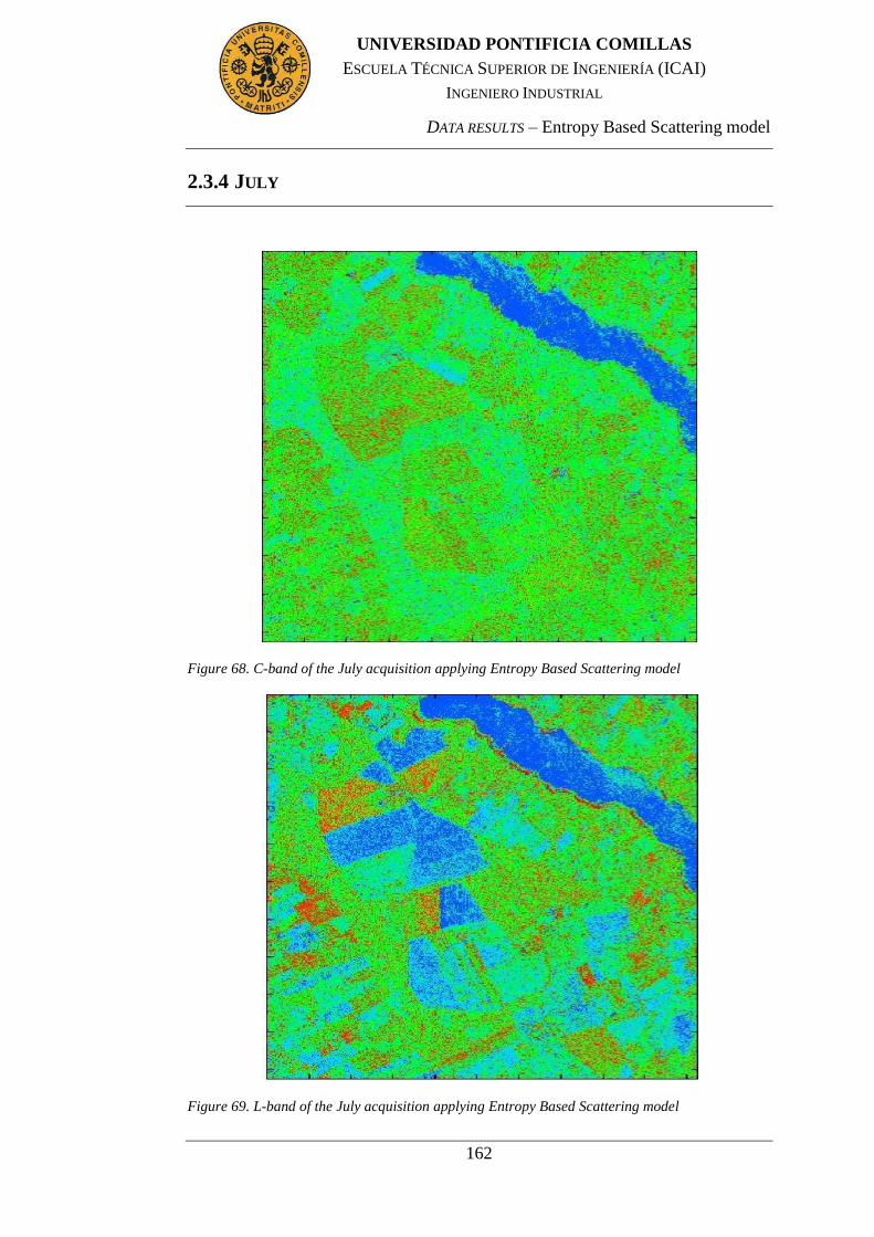
DATA RESULTS – Entropy Based Scattering model
162
UNIVERSIDAD PONTIFICIA COMILLAS
ESCUELA TÉCNICA SUPERIOR DE INGENIERÍA (ICAI)
INGENIERO INDUSTRIAL
2.3.4 JULY
Figure 68. C-band of the July acquisition applying Entropy Based Scattering model
Figure 69. L-band of the July acquisition applying Entropy Based Scattering model