
Elastic spectrum allocation in flexgrid optical networks
80
3 Universitat Politècnica de Catalunya Optical Communications Group Elastic spectrum allocation in flexgrid optical networks Adrian Asensio Garcia PROJECTE FINAL DE CARRERA Advisor: Marc Ruiz Ramírez Co-Advisor: Jaume Comellas Colomé October 2012
Transcript of Elastic spectrum allocation in flexgrid optical networks
3
Universitat Politècnica de Catalunya Optical Communications Group
Elastic spectrum allocation in flexgrid optical networks
Adrian Asensio Garcia
PROJECTE FINAL DE CARRERA
Advisor:
Marc Ruiz Ramírez
Co-Advisor:
Jaume Comellas Colomé
October 2012


3
Agraïments
En primer lloc vull agrair la dedicació i la impecable direcció d'en Marc Ruiz. Gràcies a la seva supervisió com a director del meu PFC durant tots aquests mesos, aquest projecte s'ha pogut dur a terme.
També voldria destacar l'ajut rebut en tot moment per part de la resta de membres del Grup de Comunicacions Òptiques de la UPC que no nomès m'han fet sentir com un membre més de l'equip sinò que han dedicat esforços en tot moment per tal de transmetre'm els coneixements necessaris per la realització d'aquest projecte.
Finalment, a la família i amics vull agrair-los el recolzament que m'han donat en tot moment. Especialment a la Leila i al nostre fill que està en camí, al Dani, a la Montse i al Martí.


3
Resum
En aquest treball es presenta l'estudi i els resultats obtinguts en aplicar elasticitat a xarxes òptiques flexibles amb tecnologia flexgrid amb l'objectiu d'evaluar una futura via de treball que ajudi a resoldre el problema d'enrutament i assignació d'espectre en les xarxes òptiques de propera generació.
Per dur a terme aquest projecte, es planteja un conjunt d'esquemes d'elasticitat que són avaluats per mitjà del problema de planificació de xarxa proposat, on les demandes de tràfic varien en el temps. Es proposen diverses formulacions matemàtiques i una heurística per avaluar els esquemes sobre xarxes realistes. Finalment, s'exposen conclusions sobre l’aplicació de la elasticitat al final d'aquest treball.


3
Abstract
In this work it is presented the study and the obtained results when applying elasticity in flexible optical networks using flexgrid technology and with objective to evaluate a future line of work that helps to solve the routing and spectrum allocation within next-generation optical networks.
For this project, a set of elasticity schemes is proposed and these schemes are evaluated solving the network planning problem proposed, in which traffic demands vary in time. Moreover, in order to evaluate the schemes in realistic network scenarios, both Mathematical Programming and a heuristic are proposed. Finally, the main conclusions regarding the use of elasticity are presented for concluding this work.

3
Table of Contents
List of Figures ............................................................................. XI
List of Tables ............................................................................ XIII
Chapter 1 Introduction 1 1.1 Motivation ........................................................................................................................... 1 1.2 Outline ................................................................................................................................ 2
Chapter 2 . Background 5 2.1 Optical Networks ................................................................................................................ 5 2.2 Network Management and Control ................................................................................... 9 2.3 Operational research ........................................................................................................ 11 2.4 Summary .......................................................................................................................... 13
Chapter 3 Elastic spectrum allocation 15 3.1 SA schemes ....................................................................................................................... 15 3.2 Requirements ................................................................................................................... 19
Chapter 4 Offline elastic spectrum allocation 23 4.1 Problem statement ........................................................................................................... 23 4.2 Mathematical programming ............................................................................................ 24 4.3 BRKGA heuristic .............................................................................................................. 28 4.4 Summary .......................................................................................................................... 33
Chapter 5 Illustrative numerical results 35 5.1 Network and traffic scenarios .......................................................................................... 35 5.2 Heuristics vs. ILP models ................................................................................................ 40 5.3 Evaluation of SA schemes ................................................................................................ 42 5.4 Summary .......................................................................................................................... 45

X Adrian Asensio Garcia
Chapter 6 Closing discussion 47 6.1 Contributions .................................................................................................................... 47 6.2 Future work ...................................................................................................................... 49
Appendix A. Heuristic Code 51
List of Acronyms 63
References 65
3
List of Figures
Fig. 2-1 Logical representation of a fiber optic link .................................................... 7 Fig. 2-2 RSA, continuity and contiguity constraints ................................................... 8 Fig. 2-3 Optical network planes ................................................................................. 11 Fig. 2-4 BRKGA framework (reproduced from [Go10]) ............................................. 13 Fig. 3-1 Fixed-SA scheme ........................................................................................... 16 Fig. 3-2 Underused spectrum ..................................................................................... 16 Fig. 3-3 Insufficient spectrum .................................................................................... 16 Fig. 3-4 Semi-Elastic SA - Spectrum expansion ........................................................ 17 Fig. 3-5 Semi-Elastic SA - Spectrum reduction ......................................................... 17 Fig. 3-6 Semi-Elastic SA Limitations ......................................................................... 18 Fig. 3-7 Elastic-SA with Expansion/Reduction ......................................................... 18 Fig. 3-8 Elastic-SA with reallocation ......................................................................... 19 Fig. 4-1 Spectrum allocation criteria used for the RSA algorithm ........................... 29 Fig. 4-2 Criteria for ordering demands in the RSA procedure when allocating the
last slot to transport the required bit-rate ................................................................ 30 Fig. 4-3 RSA procedure to find the initial solution ................................................... 32 Fig. 4-4 Adaptive SA procedure to improve the initial solution according to the
Semi-Elastic-SA or Elastic-SA schemes and their constraints ................................. 33 Fig. 5-1 Test Topology ................................................................................................. 36 Fig. 5-2 Spanish Telefónica (TEL) 21-node topology ................................................. 36 Fig. 5-3 British Telecom (BT) 20-node topology ........................................................ 36 Fig. 5-4 Deutsche Telekom (DT) 21-node topology .................................................... 37 Fig. 5-5 Services profiles. X-axis represents 24h of a day and Y-axis the bit-rate in
each time ...................................................................................................................... 38 Fig. 5-6 Computation time comparison ...................................................................... 41

XII Adrian Asensio Garcia
Fig. 5-7 Un-served traffic for different slot widths in the TEL topology considering
TP containing demands of only one service profile. .................................................. 43 Fig. 5-8 Un-served traffic in the TEL network topology considering TP containing
demands of different service profiles and for a slot width of 12.5 GHz ................... 43 Fig. 5-9 CF shifting (GHz) .......................................................................................... 45
3
List of Tables
Table 2-1: Spectral efficiency values for a required bandwidth of 20 GHz and
different slot widths ...................................................................................................... 9 Table 2-2: Notation for MP ......................................................................................... 11 Table 3-1: Hardware and software requirements for SA schemes ........................... 21 Table 4-1: Complexity of ILP formulations ................................................................ 28 Table 4-2: Decoder main algorithm ............................................................................ 29 Table 5-1: Capacity Parameters ................................................................................. 37 Table 5-2: Characterization of service classes. .......................................................... 38 Table 5-3: Characterization of traffic profiles. .......................................................... 39 Table 5-4: Hardware and software used for testing. ................................................. 40 Table 5-5: BRKGA parameter values. ........................................................................ 40 Table 5-6: Relative gain at UB=1% ............................................................................ 44 Table 5-7: Relative offered load gain when using Elastic-SA with spectrum
reallocation w.r.t. Elastic-SA with spectrum expansion/reduction .......................... 44 Table 6-1: Variability vs. optical technology .............................................................. 48

3
Chapter 1
Introduction
1.1 Motivation
During our day-to-day activity, it is observed that the need of connecting to the Internet is increasing and diversifying more every time. Core optical networks are able to transport high volumes of traffic by means of high-speed optical connections. The high usage of capacity of DWDM networks added to the use of upper layers to aggregate low-rate flows into the lightpaths represents the current solution to deal with such high need of data transport. Notwithstanding, traffic behavior change rapidly and the increasing mobility of traffic sources makes grooming more difficult and, therefore, the efficiency of DWDM networks is decreasing nowadays.
In light of this situation, flexgrid technology allows adapting the spectrum allocated to lightpaths to the bandwidth requirements of client demands. By dividing the spectrum in narrow slots and allowing optical connections to allocate a different number of them, the efficiency of network capacity is highly improved when comparing to DWDM networks. Thus, if future needs lead to either low-speed lightpaths with fast replacement in the network or high-speed optical connections (higher than current lightpaths in DWDM networks) to reach the optimality of data transport, flexgrid optical technology rises as the most accepted solution to substitute DWDM.
However, the basic technology of flexgrid optical networks, does not allow dynamic changes of spectrum allocation of lightpaths in a fast and easy way, fact that limits these networks to fluctuations of traffic in time. The set-up and tear-down of lightpaths generates some drawbacks that could be minimized by adapting the spectrum allocation of current established lightpaths to better match with bandwidth requirements at end points. In this regard, the application of elasticity as an elemental feature of this new optical technology is being studied and
2 Adrian Asensio Garcia
developed in research centers since it is considered as a crucial step for reaching a transport technology according to the transport requirements.
In this work, the benefits of introducing elasticity to flexgrid optical networks to carry traffic variable in time are evaluated. To this objective, several strategies to adapt the assigned spectrum of established optical connections are presented. The scenario considered to do this evaluation is a multi-hour traffic scenario, where demands of different types of services evolve in time following a specific probability distribution. The main goal of this project is to produce meaningful results and conclusions to lead the further steps of future research and to propose efficient and affordable solutions for implementing elasticity in next-generation flexgrid optical networks.
The work here presented is being developed as a part of the research objectives of the Optical Communications Group (GCO) of Universitat Politecnica de Catalunya (UPC). More specifically, this work extends the preliminary work presented in [Ve12].
1.2 Outline
The remainder of this report is as follows:
Chapter 2 introduces those necessary concepts for a good readability and comprehension of the work here presented. Specifically, the technology, management, and control of next-generation optical transport networks are presented, as well as basic concepts on operational research.
In Chapter 3 the schemes for adding elasticity to flexgrid-based optical networks are defined, focusing on the main characteristics and technological requirements to implement them in current developed flexgrid technology.
In order to evaluate the elastic schemes in Chapter 3, Chapter 4 introduces a network design problem, named MH-RSA, where traffic demands are subject to bit-rate changes in time. This problem is formulated by means of ILP formulations, one for each evaluated SA scheme. Due to the complexity of solving this problem to optimality from mathematical programming, a heuristic based on genetic algorithms is also defined.
Chapter 5 presents illustrative numerical results for, first, evaluating the quality of heuristic to obtain valid solutions for the MH-RSA problem and, second, for illustrating the performance of proposed schemes in terms of adaptability to traffic changes. Moreover, a fine analysis on those more elastic schemes is highlighted.
Finally, chapter 6 concludes this document, presenting the main contributions and conclusions of this project. Since the work here presented represents the starting point for further research works, some future steps are introduced as suggestions for extending the work.

Chapter 1 - Introduction 3
The document also contains part of the code developed in this project, regarding the implementation of the heuristic. Aiming at keeping a reasonable extension of this report, only a representative part of all the code implemented is shown.

3
Chapter 2
Background
In this Chapter, three sections are presented in order to introduce some basic concepts regarding the architecture and technology of considered optical networks, and some mathematical concepts that will be used among this work.
2.1 Optical Networks
An optical network can be defined as a network topology with its representative equipment based on a certain optical technology. In general, the edges are fiber optic links and the vertices are nodes capable of routing traffic, establishing, and deleting optical connections between source and destination nodes. Mainly the node equipment seen on this study will make reference to optical cross-connect (OXC), optical transponders (T) and wavelength selective switches (WSS). The OXC are devices capable of switching optical signals in optical networks, that is, directing an optical signal from any input port to any output port; optical transponders are the devices responsible of sending and receiving optical signals to/from a fiber optic; finally, the WSS are the equipment that integrates devices for wavelength multiplexing/demultiplexing and for switching signals per-wavelength. Since the optical technology is limited within a range of frequencies of the total frequency spectrum, the Optical Spectrum (OS) concept is introduced to define this range. The OS defines a certain capacity within the fiber optic link and it is measured in Gigahertz (GHz). In addition, this capacity depends on other factors like the equipment utilized in the nodes or the modulation format of established connections.
Another important concept deals with the optical connections established in the network. These optical connections are called lightpaths and allow the data transmission as a light wave. A fiber optic can transport more than one lightpath at the same time, since each of them is allocated in different parts of the available
6 Adrian Asensio Garcia
OS. This is the case of Dense Wavelength Division Multiplex (DWDM) networks [G.694], where the OS is divided in wavelengths and each one of them can transport at most one lightpath at the same time. This OS multiplexation allows very high capacity for transporting data in the network.
Lightpaths are responsible of serving the requested demands of customers that arrive to the network. Basically, a demand contains information about the source node (sd), the termination node (td) and the required bandwidth (or bit-rate) to be transported from the source node to the termination node, usually expressed in Megabits per second (Mbps) or Gigabits per second (Gbps). In order to establish an optical connection to serve a demand, it is necessary to solve the problem of finding a route with available free spectrum to support the lightpath. In DWDM networks, this problem is known as routing and wavelength assignment (RWA) problem.
The above described DWDM technology represents the most accepted current solution to carry with high volumes of traffic. DWDM networks are a sort of rigid optical networks, since the occupied spectrum width for all optical connections is the same (i.e. a wavelength) while the lightpath lasts active in the network. Contrarily to this definition, an elastic optical network can adapt the OS width assigned to each optical connection to the required bandwidth of the demands at each time instant. Note that in fixed optical networks it is necessary to group traffic in optical connections in order to minimize non-used resources in terms of capacity. On the other hand, elastic optical networks improve the network performance and the usage of the resources due to their adaptability in relation with the spectrum width and the spectrum allocation.
Regarding elastic optical networks, the technology that nowadays highlights among all the proposed is flexgrid [Li11]. This technology is the one that is providing the best results in terms of balance between network performance and technological complexity required for its implementation. In a flexgrid optical network (FG-ON) the OS is divided into slices, which are portions of the OS with a fixed width of few GHz (e.g. 6.25 GHz). Two consecutive slices define a slot and the central frequency (CF) defines where the assigned spectrum is centred and thus it allows positioning the slots within the whole OS. Moreover, the portion of the OS assigned to a lightpath and characterized by its CF and number of slots is called channel. In order to illustrate the concepts of optical connection, OS, CF, channel, slot, and slice, Fig 2-1 represents a fiber optic link within an elastic optical network using the flexgrid technology. In comparison with the general optical network topology seen at the beginning of this section, the FG-ON architecture requires special equipment; that is bandwidth- variable transponders (BV-T) to adjust the data signal within a CF and enough spectrum [Ge11] [Ji10] and bandwidth-variable wavelength selective switches (BV-WSS) [FINISAR] that allow to create optical routing paths having different bandwidth.

Chapter 2 - Background 7
Fig. 2-1 Logical representation of a fiber optic link
Similarly to the RWA problem, the routing and spectrum allocation (RSA) problem is solved in flexgrid networks. The objective of the RSA problem is to find a route with enough free spectrum to serve the required bandwidth for traffic demands. The spectrum allocation (SA) of an optical connection consists of finding a certain channel which must accomplish the contiguity and continuity constraints of the spectrum; that is, all slots in a channel must be one near the other (contiguity constraint) whereas the assigned channel must be placed in the same part of the OS (i.e. using the same CF) for all links conforming that optical connection (continuity constraint).
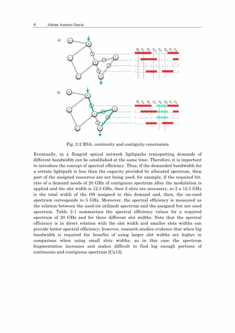
As an example of the RSA problem and for illustrating the continuity and contiguity constraints Fig 2-2 shows the routing and spectrum allocation for serving a demand with a required bit-rate equivalent to 2 slots from the source node B to the destination node D. In a first approach, illustrated in Fig.2-2a, it seems that the route B-A-D would be the one to choose as it is the shortest one. But when looking in detail, it can be seen that the links from B-A and A-D do not have two contiguous slots in the same portion of the OS and therefore the continuity and contiguity constraints are not satisfied if the route B-A-D is chosen. Because of this, another route must be selected, that is the shortest route satisfying the contiguity and continuity constraints. This is the case illustrated in Fig.2-2b, where the selected route is B-A-C-D and the assigned channel uses the slots {S5, S6} for this connection.
8 Adrian Asensio Garcia
Fig. 2-2 RSA, continuity and contiguity constraints
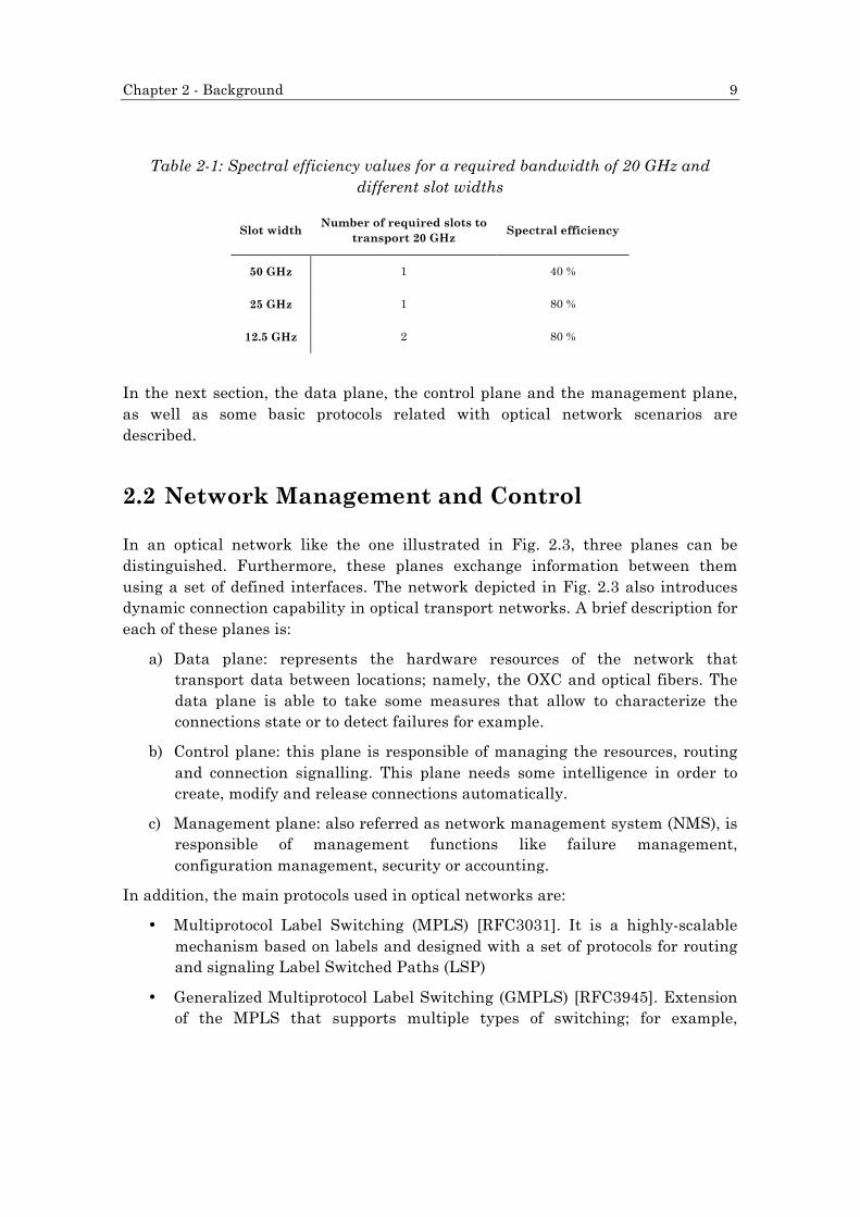
Eventually, in a flexgrid optical network ligthpaths transporting demands of different bandwidth can be established at the same time. Therefore, it is important to introduce the concept of spectral efficiency. Thus, if the demanded bandwidth for a certain lightpath is less than the capacity provided by allocated spectrum, then part of the assigned resources are not being used; for example, if the required bit-rate of a demand needs of 20 GHz of contiguous spectrum after the modulation is applied and the slot width is 12.5 GHz, then 2 slots are necessary, so 2 x 12.5 GHz is the total width of the OS assigned to this demand and, then, the un-used spectrum corresponds to 5 GHz. Moreover, the spectral efficiency is measured as the relation between the used (or utilized) spectrum and the assigned but not used spectrum. Table 2-1 summarizes the spectral efficiency values for a required spectrum of 20 GHz and for three different slot widths. Note that the spectral efficiency is in direct relation with the slot width and smaller slots widths can provide better spectral efficiency; however, research studies evidence that when big bandwidth is required the benefits of using larger slot widths are higher in comparison when using small slots widths, as in this case the spectrum fragmentation increases and makes difficult to find big enough portions of continuous and contiguous spectrum [Ca12].
Chapter 2 - Background 9
Table 2-1: Spectral efficiency values for a required bandwidth of 20 GHz and different slot widths
Slot width Number of required slots to
transport 20 GHz Spectral efficiency
50 GHz 1 40 %
25 GHz 1 80 %
12.5 GHz 2 80 %
In the next section, the data plane, the control plane and the management plane, as well as some basic protocols related with optical network scenarios are described.
2.2 Network Management and Control
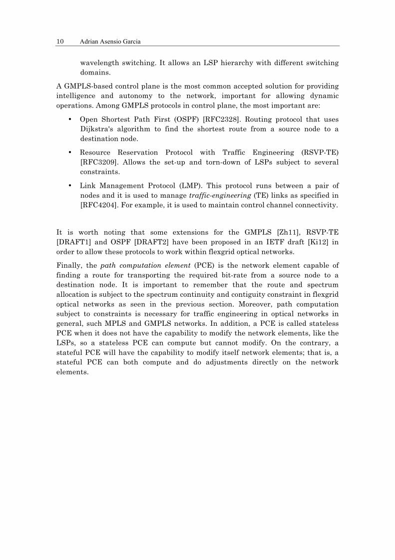
In an optical network like the one illustrated in Fig. 2.3, three planes can be distinguished. Furthermore, these planes exchange information between them using a set of defined interfaces. The network depicted in Fig. 2.3 also introduces dynamic connection capability in optical transport networks. A brief description for each of these planes is:
a) Data plane: represents the hardware resources of the network that transport data between locations; namely, the OXC and optical fibers. The data plane is able to take some measures that allow to characterize the connections state or to detect failures for example.
b) Control plane: this plane is responsible of managing the resources, routing and connection signalling. This plane needs some intelligence in order to create, modify and release connections automatically.
c) Management plane: also referred as network management system (NMS), is responsible of management functions like failure management, configuration management, security or accounting.
In addition, the main protocols used in optical networks are:
• Multiprotocol Label Switching (MPLS) [RFC3031]. It is a highly-scalable mechanism based on labels and designed with a set of protocols for routing and signaling Label Switched Paths (LSP)
• Generalized Multiprotocol Label Switching (GMPLS) [RFC3945]. Extension of the MPLS that supports multiple types of switching; for example,
10 Adrian Asensio Garcia
wavelength switching. It allows an LSP hierarchy with different switching domains.
A GMPLS-based control plane is the most common accepted solution for providing intelligence and autonomy to the network, important for allowing dynamic operations. Among GMPLS protocols in control plane, the most important are:
• Open Shortest Path First (OSPF) [RFC2328]. Routing protocol that uses Dijkstra's algorithm to find the shortest route from a source node to a destination node.
• Resource Reservation Protocol with Traffic Engineering (RSVP-TE) [RFC3209]. Allows the set-up and torn-down of LSPs subject to several constraints.
• Link Management Protocol (LMP). This protocol runs between a pair of nodes and it is used to manage traffic-engineering (TE) links as specified in [RFC4204]. For example, it is used to maintain control channel connectivity.
It is worth noting that some extensions for the GMPLS [Zh11], RSVP-TE [DRAFT1] and OSPF [DRAFT2] have been proposed in an IETF draft [Ki12] in order to allow these protocols to work within flexgrid optical networks.
Finally, the path computation element (PCE) is the network element capable of finding a route for transporting the required bit-rate from a source node to a destination node. It is important to remember that the route and spectrum allocation is subject to the spectrum continuity and contiguity constraint in flexgrid optical networks as seen in the previous section. Moreover, path computation subject to constraints is necessary for traffic engineering in optical networks in general, such MPLS and GMPLS networks. In addition, a PCE is called stateless PCE when it does not have the capability to modify the network elements, like the LSPs, so a stateless PCE can compute but cannot modify. On the contrary, a stateful PCE will have the capability to modify itself network elements; that is, a stateful PCE can both compute and do adjustments directly on the network elements.
Chapter 2 - Background 11
Data Plane
Control Plane
Management Plane
OXC
Clients
OCC
I-‐NNI
CCI
NMI-‐ANMI-‐T
OCC: Optical Connection ControllerOXC:Optical Cross-‐ConnectE-‐NNI: External Network-‐Network InterfaceI-‐NNI: Internal Network-‐Network InterfaceNMS: Network Management SystemUNI: User-‐Network InterfaceNMI-‐A: Network Management Interface – Control PlaneNMI-‐T: Network Management Interface – Data Plane
NMS
Fig. 2-3 Optical network planes
Since some mathematics is required among this study, in the next section some basic notation and concepts are presented.
2.3 Operational research
First of all, a Mathematical Programming (MP) is an exact method used to find an optimal solution of a function subject to a set of constraint [Ch83]. Formally, a general minimization problem is defined as follows:
Z*=min f (x) (2.1)
Subject to:
Ribxg ii ∈∀≥ ,)( (2.2)
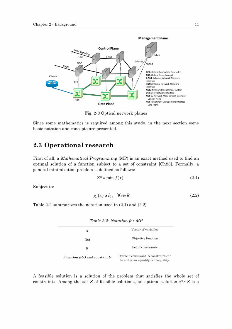
Table 2-2 summarizes the notation used in (2.1) and (2.2)
Table 2-2: Notation for MP
x Vector of variables
f(x) Objective function
R Set of constraints
Function gi(x) and constant bi Define a constraint. A constraint can be either an equality or inequality.
A feasible solution is a solution of the problem that satisfies the whole set of constraints. Among the set S of feasible solutions, an optimal solution x*ϵ S is a

12 Adrian Asensio Garcia
solution that not only satisfies the whole set of constraints but also satisfies objective function (2.1). Moreover, an optimal solution cannot be unique since there can be more than one alternative optimal solutions. However, the problem can have no feasible solutions and then it is called unfeasible. On the contrary, the problem is called unbounded if the absolute value of Z* raises to infinite.
Once introduced the basic concepts of a MP, the special case of MP called Linear Programming (LP) is presented. In a LP, f(x) and gi(x) are linear functions with real variables. In the case that the variables are restricted to be integer, the problem is called Integer Linear Programming (ILP); besides, if the problem combines both integer and real variables, then it is called Mixed Integer Linear Programming (MILP). Finally, if the problem contains, at least, one non-linear function, it is called Non-Linear Programming (NLP) [Ch83].
Another important concept deals with the complexity of a problem. If the solution of the problem is an element of a finite set of possibilities and the necessary time to verify its correctness is polynomial, then the problem is Non-deterministically Polynomial (NP). In this case, the easiest and fastest is to grade a solution instead of finding it from zero. There is a subset of the NP problems, the NP-complete. The NP-complete problems are the hardest to compute. Some basic problems within networks are NP-complete such as the RWA [Ch92] or the RSA problem described in Section 2.1. Since the complexity of RSA is higher than the one of other known network problems, the RSA problem is also defined as NP-complete. Therefore, to solve RSA problems or derivations for large (and real) instances, other methods must be used instead of applying exact solving methods. In this work, we will apply a heuristic method called Biased Random Key Genetic Algorithm (BRKGA) to solve our complex network planning problems.
The BRKGA algorithm presented by Resende in [Go10] is a genetic algorithm (GA) that can be used to efficiently solve telecommunications network planning problems. It provides near-optimal solutions in practical computational time and, in comparison with other meta-heuristics, the BRKGA provides better results in shorter running times [Go10].
The principal characteristics of genetic algorithms are:
• a chromosome composed of an array of n genes that stores each individual solution;
• each gene takes any real value within the interval [0,1];
• each chromosome encodes a solution of the problem and the value of the objective function, called fitness value;
• a population, that is, a set of individuals that evolves over a number of generations and, at each generation, they are selected and combined to generate new solutions.
Chapter 2 - Background 13
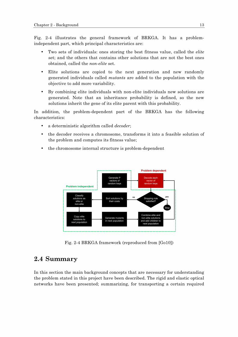
Fig. 2-4 illustrates the general framework of BRKGA. It has a problem-independent part, which principal characteristics are:
• Two sets of individuals: ones storing the best fitness value, called the elite set; and the others that contains other solutions that are not the best ones obtained, called the non-elite set.
• Elite solutions are copied to the next generation and new randomly generated individuals called mutants are added to the population with the objective to add more variability.
• By combining elite individuals with non-elite individuals new solutions are generated. Note that an inheritance probability is defined, so the new solutions inherit the gene of its elite parent with this probability.
In addition, the problem-dependent part of the BRKGA has the following characteristics:
• a deterministic algorithm called decoder;
• the decoder receives a chromosome, transforms it into a feasible solution of the problem and computes its fitness value;
• the chromosome internal structure is problem-dependent
59Computers Architecture and Networks Optimization (CANO)
Framework for BRKGA algorithms
Generate Pvectors of
random keys
Sort solutions bytheir costs
Generate mutantsin next population
Classifysolutions as
elite ornon-elite
Copy elitesolutions to
next population
Decode eachvector of
random keys
Combine elite andnon-elite solutionsand add children to
next population
Stopping rulesatisfied?
Stop
yesno
Problem independent
Problem dependent
Fig. 2-4 BRKGA framework (reproduced from [Go10])
2.4 Summary
In this section the main background concepts that are necessary for understanding the problem stated in this project have been described. The rigid and elastic optical networks have been presented; summarizing, for transporting a certain required
14 Adrian Asensio Garcia
bit-rate of a demand, in rigid optical networks the allocated part of the spectrum is fixed, independently of the required bandwidth, and thus it might be less spectrally efficient in certain scenarios such as those where the required bit-rate is lower than the allocated spectrum width. On the contrary, the elastic optical network provides mechanisms to fit the required bandwidth to the allocated spectrum width, thus increasing, the spectral efficiency. Moreover, flexgrid is described as it is the candidate technology to be applied in future elastic optical networks and the one used in this project. Basically, the flexgrid technology consists on dividing the spectrum in portions of certain width -typically 6.25GHz -, called slices; thus adding more granularity.
As it will be seen in the next chapters, it is necessary to consider combining elasticity within FG-ON, especially in scenarios where the traffic varies with the time. Next chapter describes three SA schemes with their constraints and their hardware and control plane requirements. These schemes are proposed with the intention to improve both the network performance and the spectral efficiency when applying them in realistic network scenarios that contain demands of different bit-rates and varying with time.

3
Chapter 3
Elastic spectrum allocation
Aiming at better fitting with bandwidth requirements at each moment, the lightpaths established in a network may dynamically change its allocated spectrum. This capability can be defined as elastic spectrum allocation and its implementation in future flexgrid networks is expected to provide better network performance.
In this section, three different schemes for elastic spectrum allocation in flexgrid optical networks (named SA schemes) are introduced to deal with such elasticity. Since some different hardware and control plane extensions should be considered for each scheme, a brief analysis of the requirements of SA schemes is also provided.
3.1 SA schemes
Here three elastic SA schemes are defined, focusing on the changes allowed to the allocated spectrum of lightpaths (in terms of CF and spectrum width).
3.1.1 Fixed SA
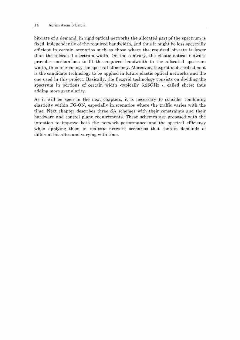
The Fixed-SA scheme, depicted in Fig 3-1, represents the case where elasticity is not allowed. Thus, under this scheme both the CF and assigned spectrum width remain static for all the time. As a consequence of this, the spectrum assignment of lightpaths is independent from variations of bandwidth requirements. Note that when comparing the requested bandwidth and the lightpath capacity, two especial situations can be distinguished:
a) When the required bandwidth is lower than the capacity of the assigned spectrum, the utilized spectrum for carrying traffic is thus lower than the allocated one, leading to a sub-optimal use of network capacity. This is the case of fig. 3-2 where the required bandwidth for the represented lightpath
16 Adrian Asensio Garcia
in time t is equal to the capacity of the assigned spectrum but the required bandwidth is lower than the capacity of the assigned spectrum in time t'.
b) When the required bandwidth is higher than the capacity of assigned spectrum, some bandwidth is not served. This is the case of fig. 3-3 where the represented lightpath has some bandwidth that is not served due to this limitation.
Allocated spectrum
Utilized spectrum
Fig. 3-1 Fixed-SA scheme
Fig. 3-2 Underused spectrum
Fig. 3-3 Insufficient spectrum
3.1.2 Semi-Elastic SA
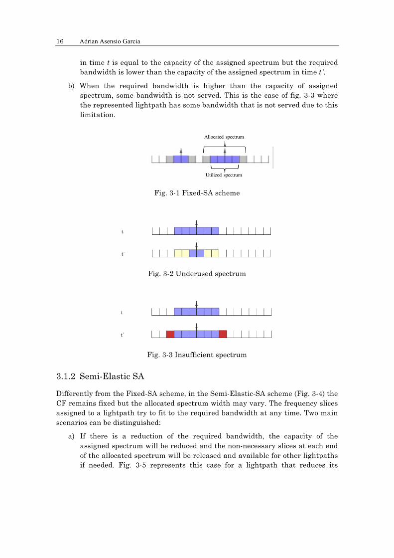
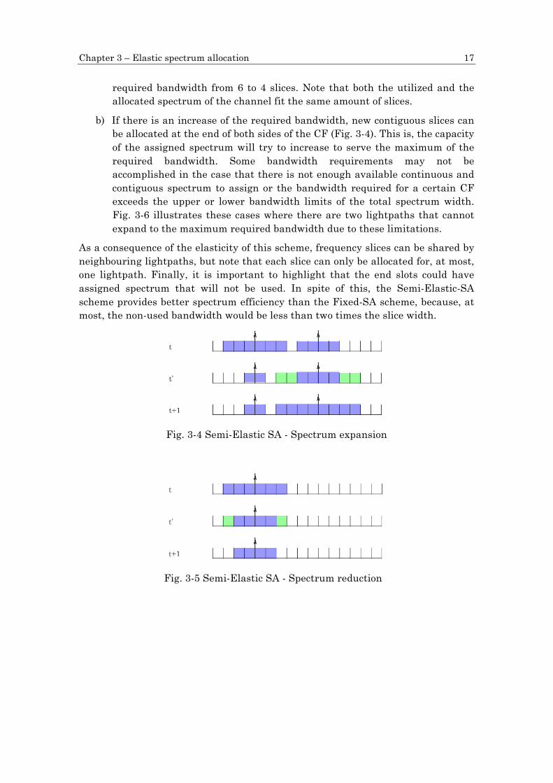
Differently from the Fixed-SA scheme, in the Semi-Elastic-SA scheme (Fig. 3-4) the CF remains fixed but the allocated spectrum width may vary. The frequency slices assigned to a lightpath try to fit to the required bandwidth at any time. Two main scenarios can be distinguished:
a) If there is a reduction of the required bandwidth, the capacity of the assigned spectrum will be reduced and the non-necessary slices at each end of the allocated spectrum will be released and available for other lightpaths if needed. Fig. 3-5 represents this case for a lightpath that reduces its
Chapter 3 – Elastic spectrum allocation 17
required bandwidth from 6 to 4 slices. Note that both the utilized and the allocated spectrum of the channel fit the same amount of slices.
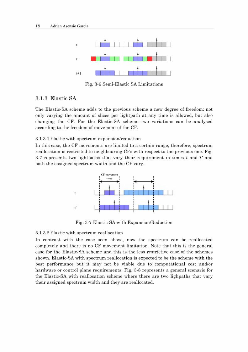
b) If there is an increase of the required bandwidth, new contiguous slices can be allocated at the end of both sides of the CF (Fig. 3-4). This is, the capacity of the assigned spectrum will try to increase to serve the maximum of the required bandwidth. Some bandwidth requirements may not be accomplished in the case that there is not enough available continuous and contiguous spectrum to assign or the bandwidth required for a certain CF exceeds the upper or lower bandwidth limits of the total spectrum width. Fig. 3-6 illustrates these cases where there are two lightpaths that cannot expand to the maximum required bandwidth due to these limitations.
As a consequence of the elasticity of this scheme, frequency slices can be shared by neighbouring lightpaths, but note that each slice can only be allocated for, at most, one lightpath. Finally, it is important to highlight that the end slots could have assigned spectrum that will not be used. In spite of this, the Semi-Elastic-SA scheme provides better spectrum efficiency than the Fixed-SA scheme, because, at most, the non-used bandwidth would be less than two times the slice width.
Fig. 3-4 Semi-Elastic SA - Spectrum expansion
Fig. 3-5 Semi-Elastic SA - Spectrum reduction
18 Adrian Asensio Garcia
Fig. 3-6 Semi-Elastic SA Limitations
3.1.3 Elastic SA
The Elastic-SA scheme adds to the previous scheme a new degree of freedom: not only varying the amount of slices per lightpath at any time is allowed, but also changing the CF. For the Elastic-SA scheme two variations can be analysed according to the freedom of movement of the CF.
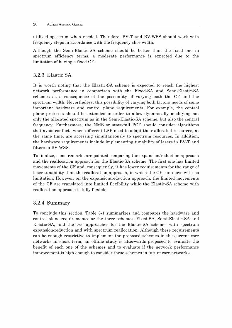
3.1.3.1 Elastic with spectrum expansion/reduction In this case, the CF movements are limited to a certain range; therefore, spectrum reallocation is restricted to neighbouring CFs with respect to the previous one. Fig. 3-7 represents two lightpaths that vary their requirement in times t and t' and both the assigned spectrum width and the CF vary.
CF movementrange
Fig. 3-7 Elastic-SA with Expansion/Reduction
3.1.3.2 Elastic with spectrum reallocation In contrast with the case seen above, now the spectrum can be reallocated completely and there is no CF movement limitation. Note that this is the general case for the Elastic-SA scheme and this is the less restrictive case of the schemes shown. Elastic-SA with spectrum reallocation is expected to be the scheme with the best performance but it may not be viable due to computational cost and/or hardware or control plane requirements. Fig. 3-8 represents a general scenario for the Elastic-SA with reallocation scheme where there are two lighpaths that vary their assigned spectrum width and they are reallocated.

Chapter 3 – Elastic spectrum allocation 19
Fig. 3-8 Elastic-SA with reallocation
3.2 Requirements
As became apparent in previous section, different requirements will be needed for each scheme. In this section, three schemes are evaluated in relation with the additional hardware and control plane extensions that would be necessary to implement them in real flexgrid networks.
3.2.1 Fixed SA
As explained above, the Fixed-SA scheme assigns to each lightpath a fixed CF and a fixed number of slices for all the time. Therefore, there are no extra hardware requirements but there are some requirements concerning the control plane extensions in order to allocate a fixed channel consisting of a fixed number of slices; extensions that have been proposed for GMPLS protocols (mainly RSVP-TE and OSPF).
Although there are no extra hardware requirements and the control plane extensions can be easily achieved, recall that the main drawback of the Fixed-SA scheme is the sub-optimal use of capacity, being the less spectrally efficient of the schemes.
3.2.2 Semi-Elastic SA
In contrast with the Fixed-SA scheme, the Semi-Elastic-SA scheme will require additional hardware adaptations. Moreover, additional control plane extensions a part of the ones required by the Fixed-SA scheme should be implemented. For example, an extension that allows modifying the current established lightpaths is needed. Since in this scheme the amount of frequency slices assigned to each lightpath is dynamically adapted, extensions of the RSVP-TE protocol should be defined in order to allow modifying the amount of slices allocated to an LSP. Also, the OSPF protocol should register slices occupancy in network links in order to provide crucial information to ensure feasible allocation decisions. Eventually, some hardware requirements should be met to allow increasing or decreasing the
20 Adrian Asensio Garcia
utilized spectrum when needed. Therefore, BV-T and BV-WSS should work with frequency steps in accordance with the frequency slice width.
Although the Semi-Elastic-SA scheme should be better than the fixed one in spectrum efficiency terms, a moderate performance is expected due to the limitation of having a fixed CF.
3.2.3 Elastic SA
It is worth noting that the Elastic-SA scheme is expected to reach the highest network performance in comparison with the Fixed-SA and Semi-Elastic-SA schemes as a consequence of the possibility of varying both the CF and the spectrum width. Nevertheless, this possibility of varying both factors needs of some important hardware and control plane requirements. For example, the control plane protocols should be extended in order to allow dynamically modifying not only the allocated spectrum as in the Semi-Elastic-SA scheme, but also the central frequency. Furthermore, the NMS or state-full PCE should consider algorithms that avoid conflicts when different LSP need to adapt their allocated resources, at the same time, are accessing simultaneously to spectrum resources. In addition, the hardware requirements include implementing tunability of lasers in BV-T and filters in BV-WSS.
To finalize, some remarks are pointed comparing the expansion/reduction approach and the reallocation approach for the Elastic-SA scheme. The first one has limited movements of the CF and, consequently, it has lower requirements for the range of laser tunability than the reallocation approach, in which the CF can move with no limitation. However, on the expansion/reduction approach, the limited movements of the CF are translated into limited flexibility while the Elastic-SA scheme with reallocation approach is fully flexible.
3.2.4 Summary
To conclude this section, Table 3-1 summarizes and compares the hardware and control plane requirements for the three schemes, Fixed-SA, Semi-Elastic-SA and Elastic-SA, and the two approaches for the Elastic-SA scheme, with spectrum expansion/reduction and with spectrum reallocation. Although these requirements can be enough restrictive to implement the proposed schemes in the current core networks in short term, an offline study is afterwards proposed to evaluate the benefit of each one of the schemes and to evaluate if the network performance improvement is high enough to consider these schemes in future core networks.

Chapter 3 – Elastic spectrum allocation 21
Table 3-1: Hardware and software requirements for SA schemes
Fixed Semi-Elastic
Elastic
With spectrum expansion/reduction
With spectrum reallocation
Hardware No extra
requirements
BV-T and BV-WSS should allow to
increase/decrease the number of allocated
slices. Spectrum tunability in
accordance with the flexgrid granularity.
Lower requirements for the range of laser
tunability than the reallocation approach.
Note that this approach has limited flexibility.
Higher requirements for the range of laser
tunability than the expansion/reduction approach. Note that this approach has
fully flexibility.
Control Plane
Extension: GMPLS, RSVP-TE, OSPF
Extension in RSVP-TE protocol to allow to
modify (increase/decrease) the
number of assigned slices
Complex algorithms in NMS/PCE to prevent conflicts during simultaneous access to
spectrum resources.

3
Chapter 4
Offline elastic spectrum allocation
To evaluate the performance of proposed SA schemes, we define a network planning problem where the expected bandwidth of demands varies in time. More specifically, we define the Multi-Hour Routing and Spectrum Allocation problem (MH-RSA), which can be solved following any of SA schemes. In order to find optimal solutions for the problem ILP formulations are introduced. However, due to the impractical use of the models in realistic networks, heuristics based on the BRKGA framework are also proposed.
4.1 Problem statement
The MH-RSA problem can be defined as follows:
Given:
• a FG-ON represented by a graph G = (N, L), where N is the set of nodes and L is the set of bidirectional fiber links;
• the same frequency spectrum for each link in L, divided into an ordered set of frequency slices S = {s1, s2,..., s|S|} of a given width and a set F = {f1, f2,...,f|F|} of central frequencies to represent the flexgrid;
• an ordered set of time intervals T = {t1, t2,...,t|T|};
• a set D of demands to be allocated in a lightpath
o sd, td: source and destination nodes of demand d.
o hdt: requested bit-rate of demand d in time interval t.
o hdmin: minimum bit-rate to be satisfied in every time interval if the demand d is accepted to the network.

24 Adrian Asensio Garcia
o hdmax: maximum bit-rate in a time period, i.e. hdmax = max {hdt, t in T}
Output:
• the SA for each time interval and the route over the FG-ON for every accepted demand.
Objective:
• minimize the number of rejected demands (primary objective). Recall that a demand is rejected if hdmin cannot be ensured in at least one time period.
• minimize the amount of un-served bit-rate (secondary objective).
Subject to
• Spectrum contiguity and continuity of lightpaths;
• A slice is allocated to only one demand at most at a given time interval;
• The allocated CF and spectrum width meet the restrictions defined for each scheme.
4.2 Mathematical programming
Because of the differences among SA schemes, defining the MH-RSA entails different formulations each one of them adapted for one scheme. However, a common notation and a set of equations can be shared for all ILPs.
4.2.1 Common notation and formulation
Before starting with the formulation, some notation is introduced as follows:
Data sets and parameters:
P Set of all paths
Pd Non-empty set of predefined candidate paths for demand d ∈ D . Each Pd comprises paths from source node sd to
destination node td
C Set of all channels
Cd Set of admissible candidate channels for demand d
Cf ⊆C Set of channels which have f ∈ F as central frequency
nc ∈ Ζ+ Number of slots forming channel c

Chapter 4 – Offline elastic spectrum allocation 25
βdct
Coefficient that represents the realized bit-rate of demand d at time interval t if channel c is selected.
h(nc ) Channel capacity
Problem variables:
xd ∈ {0,1} Binary, equal to 1 if demand d ∈ D is rejected
xp ∈ {0,1} Binary, equal to 1 if path p∈ P is selected
xpf ∈ {0,1} Binary, equal to 1 if central frequency f ∈ F is assigned to
path p∈ P
xpc ∈ {0,1} Binary, equal to 1 if channel c ∈C on path p∈ P is selected
xpct ∈ {0,1}
Binary, equal to 1 if channel c ∈C on path p∈ P is selected
in interval t ∈ T
+∈Rytd Real, with the amount of served bit-rate for demand d ∈ D in interval t ∈ T
+∈ Rvtd Real, with the amount of un-served bit-rate for demand d ∈ D in interval t ∈ T
The set of common constraints is the following:
Ddxx dPp
pd
∈∀=+∑∈
,1 (4.1)
xpct
c∈Cd :c⊃s∑
p∈Pd :p⊃l∑
d∈D∑ ≤1, ∀t ∈ T, l ∈ L, s ∈ S (4.2)
TtDdyx td
Pp Cc
tpc
tdc
d d
∈∈∀=∑∑∈ ∈
,,β (4.3)
βdct =
h nc( ), nc < ndt
hdt , nc ≥ nd
t
"
#$
%$
(4.4)
TtDdvyh td
td
td ∈∈∀=− ,, (4.5)
Constraints (4.1) deal with the path selection; whenever demand d is accepted, a path is selected from set Pd . The slice occupancy is represented by the constraints
(4.2); in a time interval a slice can be allocated to one demand at most. Constraints

26 Adrian Asensio Garcia
(4.3) represent the transported bit rate, which does not exceed the offered bit rate
and the channel capacity. There, βdct is calculated using the constraints (4.4). Note
that, although βdct coefficients are defined as part of the set of constraints, they can
be precomputed in advance as input parameters. The last constraints (4.5) deal with the un-served bit-rate calculation, computed as the difference between requested and served bit-rate.
Finally, the common function used as objective in all formulations is represented in equation (4.6), where A represents a number enough large to ensure the priority of the primary objective.
∑∑∑∈ ∈∈
⋅+⋅=Dd Tt
td
Dddd vT
xhAz 1min (4.6)
4.2.2 Fixed SA
The MH-RSA problem applying the FIXED SA scheme can be formulated as follows:
zminimize (4.7)
Subject to:
Common constraints
dp
Ccpc PpDdxx
d
∈∈∀=∑∈
,, (4.8)
TtCcPpDdxx ddpctpc ∈∈∈∈∀= ,,,, (4.9)
In this case, constraints (4.8) deal with the channel selection on the active routing path; whereas constraints (4.9) guarantee that the channel is used in each time interval.
4.2.3 Semi-Elastic SA
When applying this scheme, the problem should be defined according to the next formulation:
zminimize
Subject to:
Common constraints
Ppxx pFf
pf ∈∀=∑∈
, (4.10)

Chapter 4 – Offline elastic spectrum allocation 27
TtFfPpDdxx dpfCCc
tpcdf
∈∈∈∈∀=∑∩∈
,,,, (4.11)
Here, constraints (4.10) select a CF on the active routing path and constraints (4.11) select a channel of this CF for each time period.
4.2.4 Elastic SA with Expansion/Reduction
The specific notation for the Elastic SA allowing only expansions and reductions within a limited range is:
zminimize (4.12)
Subject to:
Common constraints
TtPpDdxx dpCc
tpc
d
∈∈∈∀=∑∈
,,, (4.13)
SsTtPpDdnnxx dt
d
td
scCc
tpc
scCc
tpc
dd
∈∈∈∈∀Δ+
≤−+
⊃∈
+
⊃∈∑∑ ,,,,1:
1
:
(4.14)
xpct+1
c∈Cd :c⊃s∑ − xpc
t
c∈Cd :c⊃s∑ ≤
ndt+1
ndt +Δ
, ∀d ∈ D, p∈ Pd, t ∈ T, s ∈ S (4.15)
In this scheme, constraints (4.13) select a channel within the active routing path for each time period. Moreover, constraints (4.14) represent expansion constraints, whereas constraints (4.15) are the reduction constraints.
4.2.5 Elastic SA with Reallocation
Finally, when allowing lightpath reallocation to any part of the spectrum, the Elastic SA schemes is modeled as follows:
zminimize (4.16)
Subject to:
Common constraints
TtPpDdxx dpCc
tpc
d
∈∈∈∀=∑∈
,,, (4.17)
In addition to common constraints, constraints (4.17) select a channel on the active routing path for each time period, as the constraints (4.13) do.
28 Adrian Asensio Garcia
4.2.6 Complexity analysis
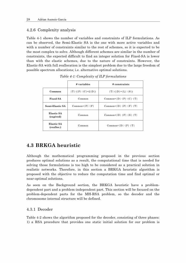
Table 4-1 shows the number of variables and constraints of ILP formulations. As can be observed, the Semi-Elastic SA is the one with more active variables and with a number of constraints similar to the rest of schemes, so it is expected to be the most complex to solve. Although different schemes are similar in the number of constraints, the expected difficult to find an integer solution for Fixed-SA is lower than with the elastic schemes, due to the nature of constraints. However, the Elastic-SA with full reallocation is the simplest problem due to the large freedom of possible spectrum allocations; i.e. alternative optimal solutions.
Table 4-1: Complexity of ILP formulations
# variables # constraints
Common |T|·(|P|·|C|+2|D|) |T|·(|D|+|L|·|S|)
Fixed SA Common Common+|D|·|P|·|C|·|T|
Semi-Elastic SA Common+|P|·|F| Common+|D|·|P|·|F|·|T|
Elastic SA (exp/red)
Common Common+|D|·|P|·|S|·|T|
Elastic SA (realloc.)
Common Common+|D|·|P|·|T|
4.3 BRKGA heuristic
Although the mathematical programming proposed in the previous section produces optimal solutions as a result, the computational time that is needed for solving those formulations is too high to be considered as a practical solution in realistic networks. Therefore, in this section a BRKGA heuristic algorithm is proposed with the objective to reduce the computation time and find optimal or near-optimal solutions.
As seen on the Background section, the BRKGA heuristic have a problem-dependent part and a problem-independent part. This section will be focused on the problem-dependent parts for the MH-RSA problem, so the decoder and the chromosome internal structure will be defined.
4.3.1 Decoder
Table 4-2 shows the algorithm proposed for the decoder, consisting of three phases: 1) a RSA procedure that provides one static initial solution for our problem is
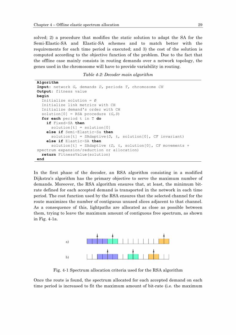
Chapter 4 – Offline elastic spectrum allocation 29
solved; 2) a procedure that modifies the static solution to adapt the SA for the Semi-Elastic-SA and Elastic-SA schemes and to match better with the requirements for each time period is executed; and 3) the cost of the solution is computed according to the objective function of the problem. Due to the fact that the offline case mainly consists in routing demands over a network topology, the genes used in the chromosome will have to provide variability in routing.
Table 4-2: Decoder main algorithm
Algorithm Input: network G, demands D, periods T, chromosome CH Output: fitness value begin Initialize solution = Ø Initialize link metrics with CH Initialize demand's order with CH solution[0] = RSA procedure (G,D) for each period t in T do if Fixed-SA then solution[t] = solution[0] else if Semi-Elastic-Sa then solution[t] = SAdaptive(D, t, solution[0], CF invariant) else if Elastic-SA then solution[t] = SAdaptive (D, t, solution[0], CF movements + spectrum expansion/reduction or allocation) return FitnessValue(solution) end
In the first phase of the decoder, an RSA algorithm consisting in a modified Dijkstra's algorithm has the primary objective to serve the maximum number of demands. Moreover, the RSA algorithm ensures that, at least, the minimum bit-rate defined for each accepted demand is transported in the network in each time period. The cost function used by the RSA ensures that the selected channel for the route maximizes the number of contiguous unused slices adjacent to that channel. As a consequence of this, lightpaths are allocated as close as possible between them, trying to leave the maximum amount of contiguous free spectrum, as shown in Fig. 4-1a.
Fig. 4-1 Spectrum allocation criteria used for the RSA algorithm
Once the route is found, the spectrum allocated for each accepted demand on each time period is increased to fit the maximum amount of bit-rate (i.e. the maximum
30 Adrian Asensio Garcia
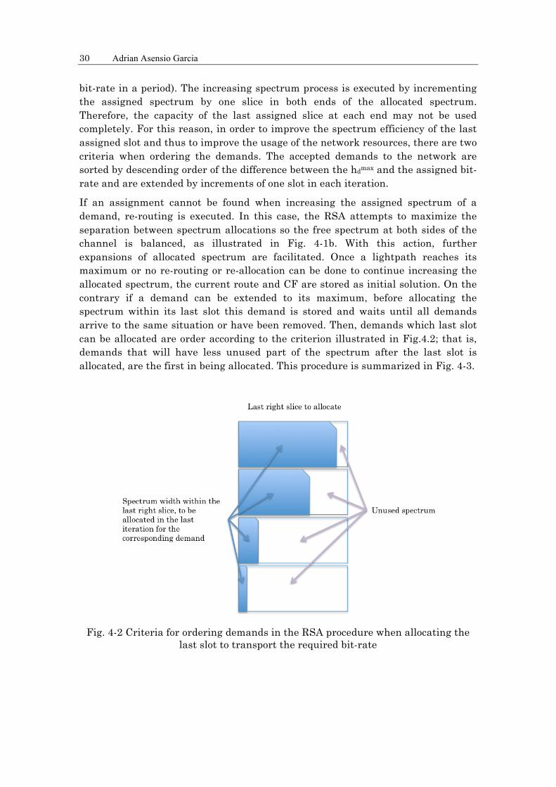
bit-rate in a period). The increasing spectrum process is executed by incrementing the assigned spectrum by one slice in both ends of the allocated spectrum. Therefore, the capacity of the last assigned slice at each end may not be used completely. For this reason, in order to improve the spectrum efficiency of the last assigned slot and thus to improve the usage of the network resources, there are two criteria when ordering the demands. The accepted demands to the network are sorted by descending order of the difference between the hdmax and the assigned bit-rate and are extended by increments of one slot in each iteration.
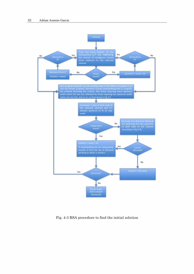
If an assignment cannot be found when increasing the assigned spectrum of a demand, re-routing is executed. In this case, the RSA attempts to maximize the separation between spectrum allocations so the free spectrum at both sides of the channel is balanced, as illustrated in Fig. 4-1b. With this action, further expansions of allocated spectrum are facilitated. Once a lightpath reaches its maximum or no re-routing or re-allocation can be done to continue increasing the allocated spectrum, the current route and CF are stored as initial solution. On the contrary if a demand can be extended to its maximum, before allocating the spectrum within its last slot this demand is stored and waits until all demands arrive to the same situation or have been removed. Then, demands which last slot can be allocated are order according to the criterion illustrated in Fig.4.2; that is, demands that will have less unused part of the spectrum after the last slot is allocated, are the first in being allocated. This procedure is summarized in Fig. 4-3.
Fig. 4-2 Criteria for ordering demands in the RSA procedure when allocating the last slot to transport the required bit-rate

Chapter 4 – Offline elastic spectrum allocation 31
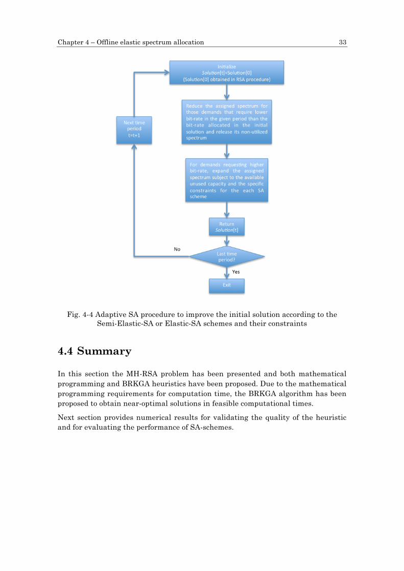
In the second phase the initial solution provided by the RSA procedure is used to compute time-period dependent solutions. For the Fixed-SA scheme, the static solution remains fixed for all the time periods whereas for the Semi-Elastic-SA and for the Elastic-SA an adaptive SA procedure varies the static solution taking into account the constraints for these schemes regarding the expansion/reduction of the assigned spectrum and the variations of the CF. To modify the static solution there are two steps for each time period as illustrated in Fig. 4-4. In the first step, the proposed algorithm releases the allocated slices for the demands that require lower bit-rate than the one allocated in initial solution. Therefore, more free spectrum is available for the demands that require higher bandwidth than the provided by the allocated spectrum. These demands are processed in the second step, where the algorithm tries to expand the assigned spectrum subject to the available unused capacity and the specific constraints for the each SA scheme. Finally, the fitness value of the solution is computed following the objective function defined in each formulation.
4.3.2 Chromosome
As seen on the decoder definition, a RSA is used to obtain the static solution. To add variability in routing, one gene for each link is needed, containing the link weight. Thus, the metric of the link is obtained by multiplying the link distance by the random link weight. Then, the resultant metrics are used to compute shortest paths in the modified Dijkstra's algorithm. Moreover, the order in which the demands are processed affects directly to the quality of the obtained initial solution. Therefore, it is reasonable to use another gene to code the order to process the demands. Taking this into account, the chromosomes can be defined as arrays of m = |D|+|E| genes.
32 Adrian Asensio Garcia
Fig. 4-3 RSA procedure to find the initial solution
Chapter 4 – Offline elastic spectrum allocation 33
Fig. 4-4 Adaptive SA procedure to improve the initial solution according to the Semi-Elastic-SA or Elastic-SA schemes and their constraints
4.4 Summary
In this section the MH-RSA problem has been presented and both mathematical programming and BRKGA heuristics have been proposed. Due to the mathematical programming requirements for computation time, the BRKGA algorithm has been proposed to obtain near-optimal solutions in feasible computational times.
Next section provides numerical results for validating the quality of the heuristic and for evaluating the performance of SA-schemes.

3
Chapter 5
Illustrative numerical results
In previous Chapters, the Fixed-SA, the Semi-Elastic-SA and the Elastic-SA schemes have been defined and the offline MH-RSA problem has been stated. Moreover, both ILPs and BRKGA algorithm have been proposed to solve it. Therefore, in order to evaluate the schemes proposed and the quality of the solutions obtained with the heuristic, some numerical results will be provided in this Chapter.
Three sections can be distinguished. First of all, the network and the traffic scenarios considered in the offline problem will be defined. After that, and before using the heuristics to execute the simulations, the quality of the BRKGA algorithm will be validated by comparing the obtained solutions with the optimal ones obtained by solving the ILP formulations introduced in Chapter 4. Finally, in order to compare the effectiveness of the schemes proposed, the heuristics will be used to carry out exhaustive experiments.
5.1 Network and traffic scenarios
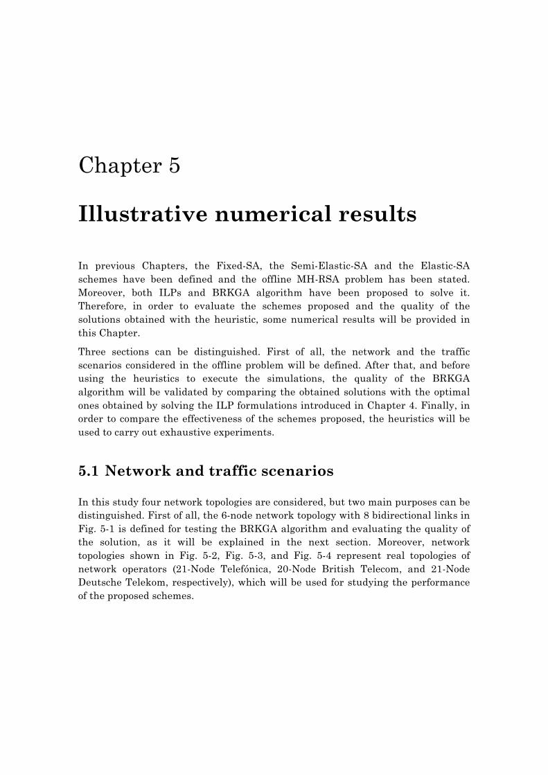
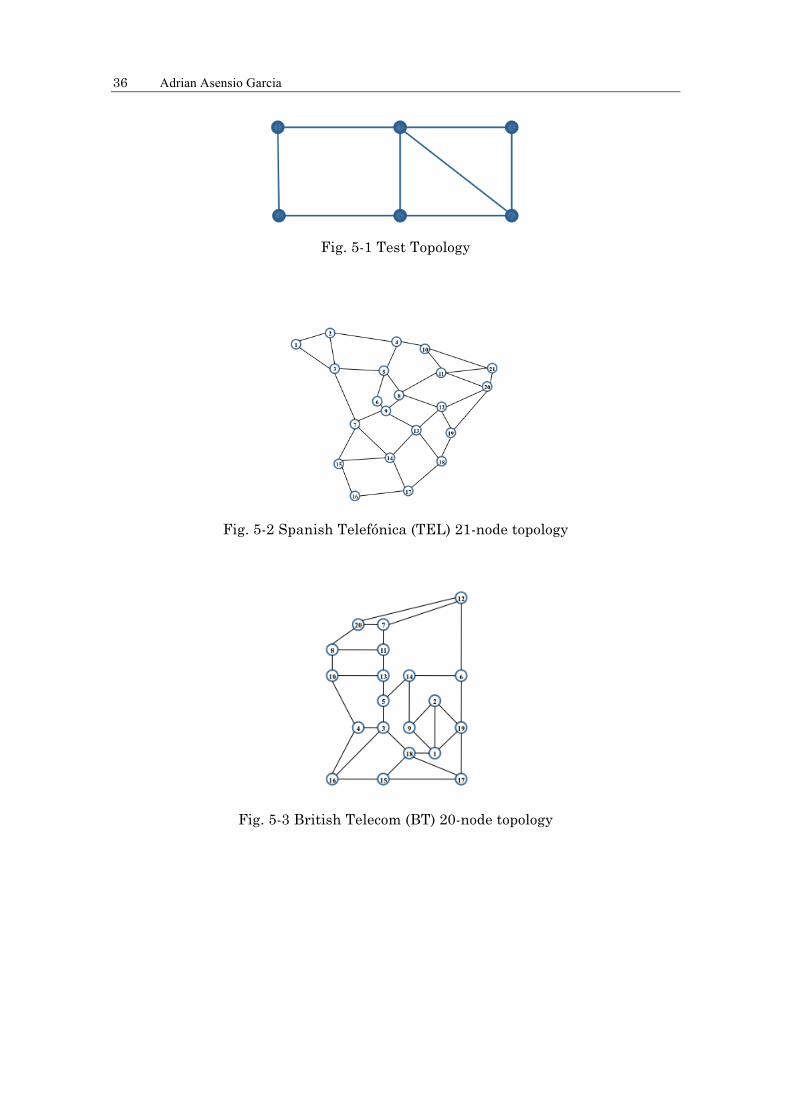
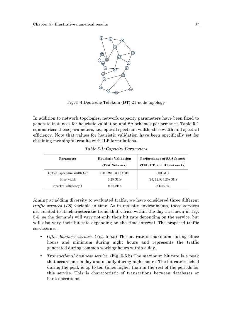
In this study four network topologies are considered, but two main purposes can be distinguished. First of all, the 6-node network topology with 8 bidirectional links in Fig. 5-1 is defined for testing the BRKGA algorithm and evaluating the quality of the solution, as it will be explained in the next section. Moreover, network topologies shown in Fig. 5-2, Fig. 5-3, and Fig. 5-4 represent real topologies of network operators (21-Node Telefónica, 20-Node British Telecom, and 21-Node Deutsche Telekom, respectively), which will be used for studying the performance of the proposed schemes.
36 Adrian Asensio Garcia
Fig. 5-1 Test Topology
Fig. 5-2 Spanish Telefónica (TEL) 21-node topology
Fig. 5-3 British Telecom (BT) 20-node topology
Chapter 5 - Illustrative numerical results 37
Fig. 5-4 Deutsche Telekom (DT) 21-node topology
In addition to network topologies, network capacity parameters have been fixed to generate instances for heuristic validation and SA schemes performance. Table 5-1 summarizes these parameters, i.e., optical spectrum width, slice width and spectral efficiency. Note that values for heuristic validation have been specifically set for obtaining meaningful results with ILP formulations.
Table 5-1: Capacity Parameters
Parameter Heuristic Validation
(Test Network)
Performance of SA Schemes
(TEL, BT, and DT networks)
Optical spectrum width OS {100, 200, 300} GHz 800 GHz
Slice width 6.25 GHz (25, 12.5, 6.25) GHz
Spectral efficiency I 2 bits/Hz 2 bits/Hz
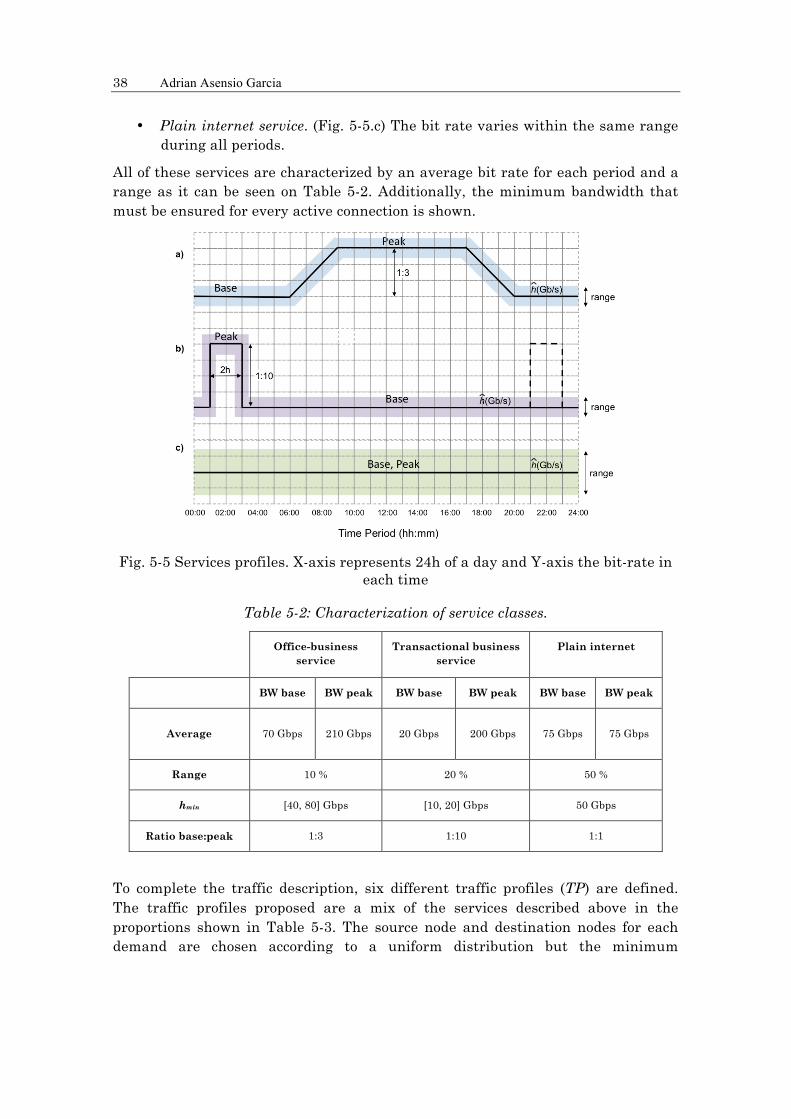
Aiming at adding diversity to evaluated traffic, we have considered three different traffic services (TS) variable in time. As in realistic environments, these services are related to its characteristic trend that varies within the day as shown in Fig. 5-5, so the demands will vary not only their bit rate depending on the service, but will also vary their bit rate depending on the time interval. The proposed traffic services are:
• Office-business service. (Fig. 5-5.a) The bit rate is maximum during office hours and minimum during night hours and represents the traffic generated during common working hours within a day.
• Transactional business service. (Fig. 5-5.b) The maximum bit rate is a peak that occurs once a day and usually during night hours. The bit rate reached during the peak is up to ten times higher than in the rest of the periods for this service. This is characteristic of transactions between databases or bank operations.
38 Adrian Asensio Garcia
• Plain internet service. (Fig. 5-5.c) The bit rate varies within the same range during all periods.
All of these services are characterized by an average bit rate for each period and a range as it can be seen on Table 5-2. Additionally, the minimum bandwidth that must be ensured for every active connection is shown.
Fig. 5-5 Services profiles. X-axis represents 24h of a day and Y-axis the bit-rate in each time
Table 5-2: Characterization of service classes.
Office-business service
Transactional business service
Plain internet
BW base BW peak BW base BW peak BW base BW peak
Average 70 Gbps 210 Gbps 20 Gbps 200 Gbps 75 Gbps 75 Gbps
Range 10 % 20 % 50 %
hmin [40, 80] Gbps [10, 20] Gbps 50 Gbps
Ratio base:peak 1:3 1:10 1:1
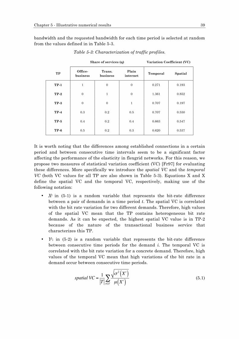
To complete the traffic description, six different traffic profiles (TP) are defined. The traffic profiles proposed are a mix of the services described above in the proportions shown in Table 5-3. The source node and destination nodes for each demand are chosen according to a uniform distribution but the minimum
Chapter 5 - Illustrative numerical results 39
bandwidth and the requested bandwidth for each time period is selected at random from the values defined in in Table 5-3.
Table 5-3: Characterization of traffic profiles.
Share of services (q) Variation Coefficient (VC)
TP Office-
business Trans.
business Plain
internet Temporal Spatial
TP-1 1 0 0 0.271 0.193
TP-2 0 1 0 1.361 0.852
TP-3 0 0 1 0.707 0.197
TP-4 0.3 0.2 0.5 0.707 0.550
TP-5 0.4 0.2 0.4 0.663 0.547
TP-6 0.5 0.2 0.3 0.620 0.537
It is worth noting that the differences among established connections in a certain period and between consecutive time intervals seem to be a significant factor affecting the performance of the elasticity in flexgrid networks. For this reason, we propose two measures of statistical variation coefficient (VC) [Fr97] for evaluating these differences. More specifically we introduce the spatial VC and the temporal VC (both VC values for all TP are also shown in Table 5-3). Equations X and X define the spatial VC and the temporal VC, respectively, making use of the following notation:
• Xt in (5-1) is a random variable that represents the bit-rate difference between a pair of demands in a time period t. The spatial VC is correlated with the bit rate variation for two different demands. Therefore, high values of the spatial VC mean that the TP contains heterogeneous bit rate demands. As it can be expected, the highest spatial VC value is in TP-2 because of the nature of the transactional business service that characterizes this TP.
• Yti in (5-2) is a random variable that represents the bit-rate difference between consecutive time periods for the demand i. The temporal VC is correlated with the bit rate variation for a concrete demand. Therefore, high values of the temporal VC mean that high variations of the bit rate in a demand occur between consecutive time periods.
spatial VC = 1T
σ 2 Xt( )µ Xt( )t∈T
∑ (5.1)

40 Adrian Asensio Garcia
temporal VC = 1T −1
qii∈TS∑
σ 2 Y t( )µ Y t( )t∈T−{tT }
∑ (5.2)
5.2 Heuristics vs. ILP models
Table 5-4 summarizes the hardware and software used for solving the problem and for obtaining the results shown in this section. Details of the implementation of the BRKGA heuristic in Matlab® can be found in Appendix A. Recall that the Elastic-SA used for this comparison is the one with spectrum allocation.
Table 5-4: Hardware and software used for testing.
ILP models BRKGA heuristics
Software CPLEX v.12.2 optimizer
[CPLEX] Matlab® [MATLAB]
Hardware 2.4 GHz Quad-core
8 GB RAM
Aiming at evaluating the quality of heuristics, we have randomly generated 50 instances containing a number of demands |D| in the range [3, 15]. All instances were solved with capacity parameters in Table 5-1 and for a number of time intervals |T|= {3, 6, 12}. Due to the difficulty of obtaining exact values, we have limited our tests to traffic following TP-3. Before comparing ILP and heuristic solutions, we have solved all these instances with our BRKGA implementation for a wide range of values for tuneable parameters. Table 5-5 summarizes the best parameter configuration according to the results of these tests. Without loss of generality, we have applied that configuration for real instances in next subsection, since these values are in accordance with similar studies [Ru11].
Table 5-5: BRKGA parameter values.
length of the chromosome (m) |E| + |D|
population size (p) min(75, m)
elite population size 0.2 · p
mutant population size 0.2 · p
elite inheritance probability 0.7
After heuristic tuning we have compared the results of ILP and heuristics for those test instances that were solved to optimality. The quality of our BRKGA heuristic can be evaluated based on the following results:
Chapter 5 - Illustrative numerical results 41
• Heuristic founds the optimal solution in more than 95% of the instances.
• Heuristic founds near-optimal solutions with a worst gap compared with ILP model below 3%.
• The on-average optimality gap of heuristic remains below 0.1%
Moreover, a high improvement in the computational time is achieved (as expected) according to the following:
• Heuristic best solutions obtained in less than 50 seconds in average (few minutes for the largest instances)
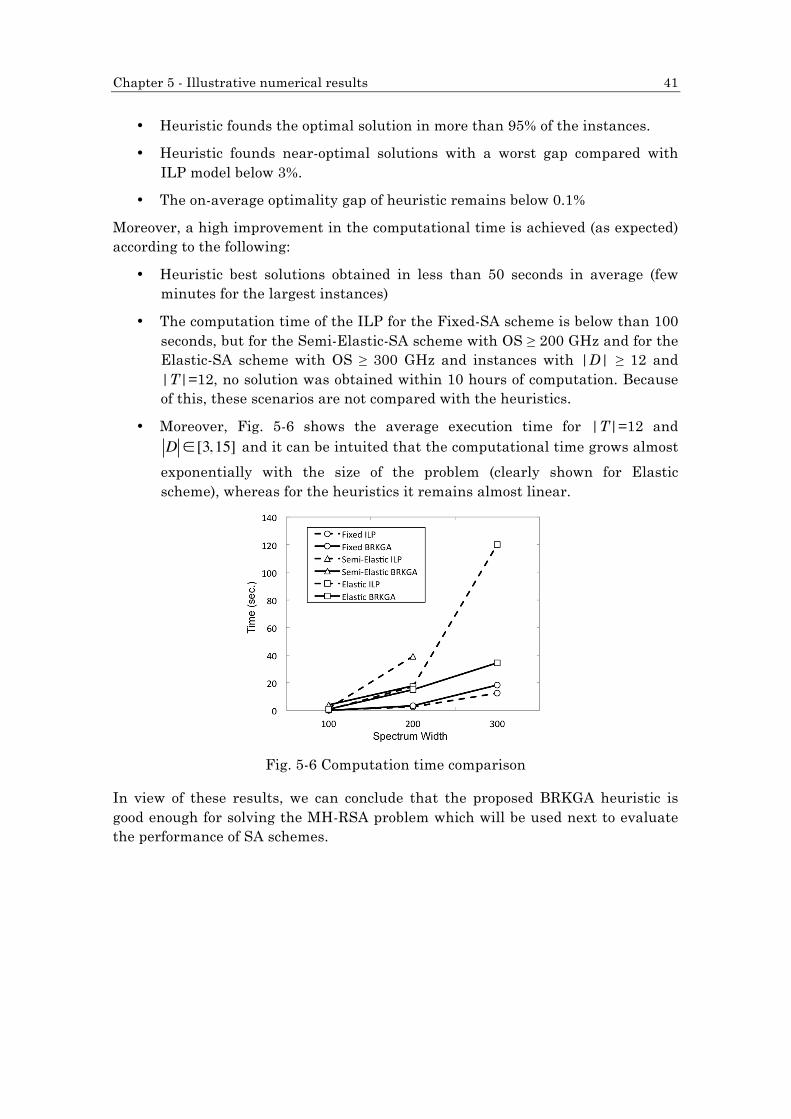
• The computation time of the ILP for the Fixed-SA scheme is below than 100 seconds, but for the Semi-Elastic-SA scheme with OS ≥ 200 GHz and for the Elastic-SA scheme with OS ≥ 300 GHz and instances with |D| ≥ 12 and |T|=12, no solution was obtained within 10 hours of computation. Because of this, these scenarios are not compared with the heuristics.
• Moreover, Fig. 5-6 shows the average execution time for |T|=12 and D ∈ [3, 15] and it can be intuited that the computational time grows almost
exponentially with the size of the problem (clearly shown for Elastic scheme), whereas for the heuristics it remains almost linear.
Fig. 5-6 Computation time comparison
In view of these results, we can conclude that the proposed BRKGA heuristic is good enough for solving the MH-RSA problem which will be used next to evaluate the performance of SA schemes.
42 Adrian Asensio Garcia
5.3 Evaluation of SA schemes
In this section the results and the performance of each of the schemes proposed will be analysed in the realistic network scenarios. Therefore, the set of demands of each generated instance will be large enough to be comparable to real traffic levels.
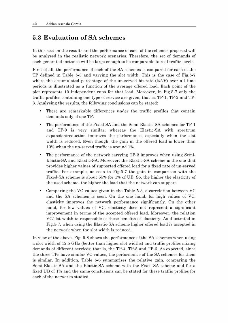
First of all, the performance of each of the SA schemes is compared for each of the TP defined in Table 5-3 and varying the slot width. This is the case of Fig.5-7 where the accumulated percentage of the un-served bit-rate (%UB) over all time periods is illustrated as a function of the average offered load. Each point of the plot represents 10 independent runs for that load. Moreover, in Fig.5-7 only the traffic profiles containing one type of service are given, that is, TP-1, TP-2 and TP-3. Analysing the results, the following conclusions can be stated:
• There are remarkable differences under the traffic profiles that contain demands only of one TP.
• The performance of the Fixed-SA and the Semi-Elastic-SA schemes for TP-1 and TP-3 is very similar; whereas the Elastic-SA with spectrum expansion/reduction improves the performance, especially when the slot width is reduced. Even though, the gain in the offered load is lower than 10% when the un-served traffic is around 1%.
• The performance of the network carrying TP-2 improves when using Semi-Elastic-SA and Elastic-SA. Moreover, the Elastic-SA scheme is the one that provides higher values of supported offered load for a fixed rate of un-served traffic. For example, as seen in Fig.5-7 the gain in comparison with the Fixed-SA scheme is about 55% for 1% of UB. So, the higher the elasticity of the used scheme, the higher the load that the network can support.
• Comparing the VC values given in the Table 5-3, a correlation between VC and the SA schemes is seen. On the one hand, for high values of VC, elasticity improves the network performance significantly. On the other hand, for low values of VC, elasticity does not represent a significant improvement in terms of the accepted offered load. Moreover, the relation VC/slot width is responsible of these benefits of elasticity. As illustrated in Fig.5-7, when using the Elastic-SA scheme higher offered load is accepted in the network when the slot width is reduced.
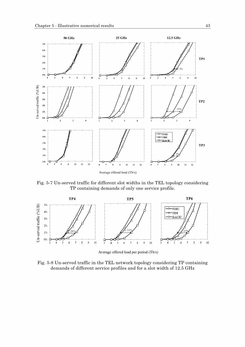
In view of the above, Fig. 5-8 shows the performance of the SA schemes when using a slot width of 12.5 GHz (better than higher slot widths) and traffic profiles mixing demands of different services; that is, the TP-4, TP-5 and TP-6. As expected, since the three TPs have similar VC values, the performance of the SA schemes for them is similar. In addition, Table 5-6 summarizes the relative gain, comparing the Semi-Elastic-SA and the Elastic-SA scheme with the Fixed-SA scheme and for a fixed UB of 1% and the same conclusions can be stated for these traffic profiles for each of the networks studied.
Chapter 5 - Illustrative numerical results 43
Fig. 5-7 Un-served traffic for different slot widths in the TEL topology considering TP containing demands of only one service profile.
Fig. 5-8 Un-served traffic in the TEL network topology considering TP containing demands of different service profiles and for a slot width of 12.5 GHz

44 Adrian Asensio Garcia
Table 5-6: Relative gain at UB=1%
TP Semi-Elastic w.r.t Fixed
Elastic w.r.t Fixed
TEL
TP4 3.52 % 28.31 %
TP5 4.71 % 30.79 %
TP6 8.40 % 27.30 %
BT
TP4 8.32 % 29.19 %
TP5 4.67 % 27.29 %
TP6 15.14 % 29.98 %
DT
TP4 2.39 % 16.90 %
TP5 2.02 % 16.70 %
TP6 8.82 % 16.59 %
5.3.1 Comparison of the Elastic approaches
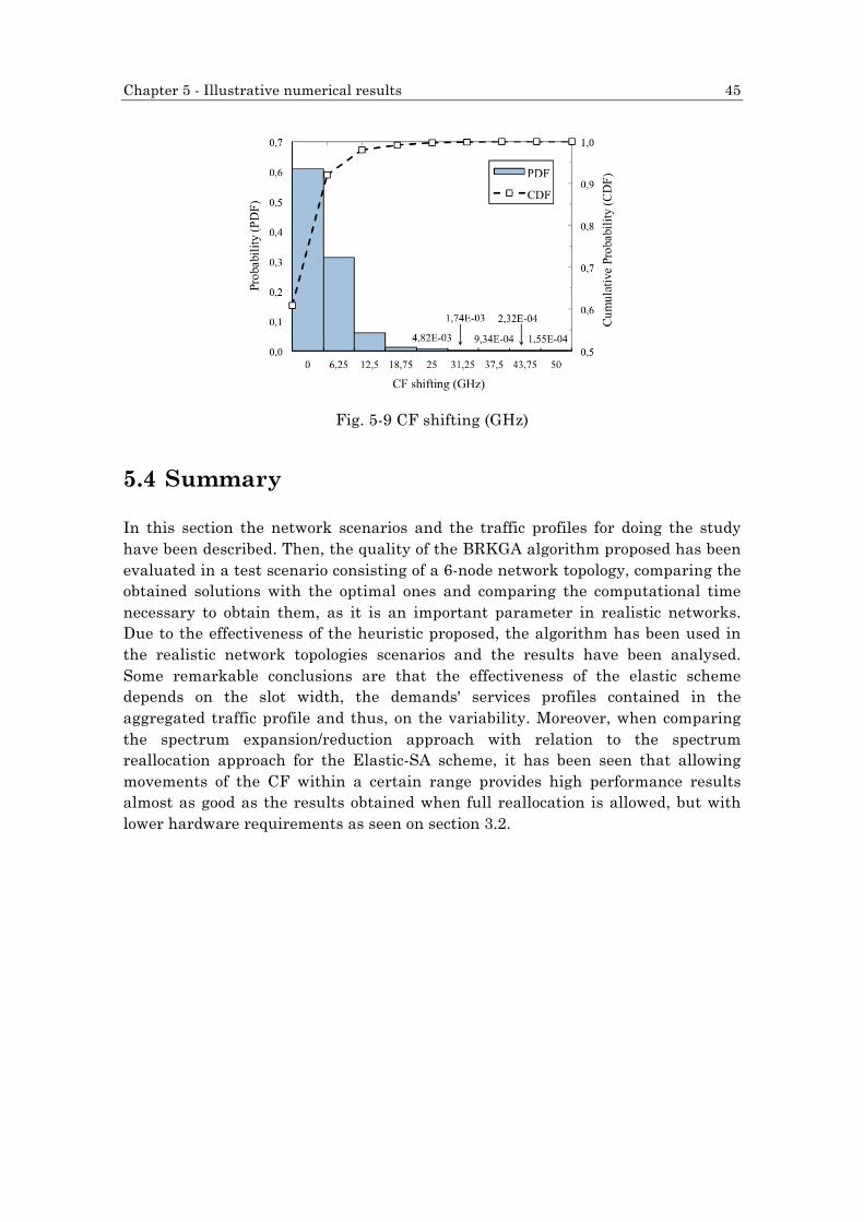
It is worth noting that the Elastic-SA scheme studied in this section is the approach with spectrum expansion/reduction. Table 5-7 summarizes the relative gain in comparison with the spectrum reallocation approach in terms of offered load when the UB is equal to 1%. Furthermore, as seen in Fig. 5-9, if the allowed variation width for the CF is 12.5 GHz in the Elastic-SA scheme with spectrum expansion/reduction, the network performance is quite similar that in the case of Elastic-SA with spectrum reallocation. Therefore, the Elastic-SA with spectrum expansion/reduction is a feasible solution to exploit elasticity in flexgrid networks.
Table 5-7: Relative offered load gain when using Elastic-SA with spectrum reallocation w.r.t. Elastic-SA with spectrum expansion/reduction
Network TP Offered load gain
TEL
TP-4 1.45 %
TP-5 0.95 %
TP-6 0.14 %
BT
TP-4 3.62 %
TP-5 1.29 %
TP-6 0.84 %
DT
TP-4 4.90 %
TP-5 4.01 %
TP-6 0.54 %
Chapter 5 - Illustrative numerical results 45
Fig. 5-9 CF shifting (GHz)
5.4 Summary
In this section the network scenarios and the traffic profiles for doing the study have been described. Then, the quality of the BRKGA algorithm proposed has been evaluated in a test scenario consisting of a 6-node network topology, comparing the obtained solutions with the optimal ones and comparing the computational time necessary to obtain them, as it is an important parameter in realistic networks. Due to the effectiveness of the heuristic proposed, the algorithm has been used in the realistic network topologies scenarios and the results have been analysed. Some remarkable conclusions are that the effectiveness of the elastic scheme depends on the slot width, the demands' services profiles contained in the aggregated traffic profile and thus, on the variability. Moreover, when comparing the spectrum expansion/reduction approach with relation to the spectrum reallocation approach for the Elastic-SA scheme, it has been seen that allowing movements of the CF within a certain range provides high performance results almost as good as the results obtained when full reallocation is allowed, but with lower hardware requirements as seen on section 3.2.

3
Chapter 6
Closing discussion
In this chapter, the main contributions of this study are summarized and future work is presented, as the results described in this work are the first step for deeper studies in flexgrid optical networks (e.g., in online scenarios). Finally, the list of references closes this chapter.
6.1 Contributions
An important problem affecting the deployment of the flexgrid optical technology is the increasing presence of traffic variable in the time. Although rigid flexgrid solutions are valid for scenarios where heterogeneous traffic remains invariable during holding time of connections, they lack of adaptability when required bit-rate varies. To add elasticity to flexgrid optical networks, three schemes with different degrees of adaptability were introduced. These schemes are: the Fixed-SA scheme, in which a fixed part of the spectrum is allocated for each demand independently of the required bit-rate; the Semi-Elastic-SA scheme, in which for a fixed CF the width of the allocated spectrum can be expanded or reduced in order to fit the required bit-rate of the demands in each time period; and the Elastic-SA scheme, in which movements of the CF are allowed. Furthermore, for the Elastic-SA two cases are distinguished depending on the freedom of movements of the CF: the Elastic-SA with spectrum expansion/reduction, where the CF can move within a range of frequencies; and the Elastic-SA with spectrum reallocation that has no limitations regarding the movements of the CF within the whole OS.
To evaluate the performance of SA elasticity schemes, the MH-RSA problem was introduced as a network planning problem and several ILP formulations were presented. Due to the large computational time required to find optimal solutions from ILPs, the BRKGA heuristic is proposed. After solving several instances in a test network, both the quality of solutions and the affordability of execution times were validated. In addition, three realistic network topologies (TEL, BT and DT) are described and different traffic profiles are defined. The traffic profiles contain
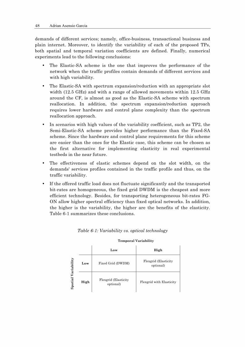
48 Adrian Asensio Garcia
demands of different services; namely, office-business, transactional business and plain internet. Moreover, to identify the variability of each of the proposed TPs, both spatial and temporal variation coefficients are defined. Finally, numerical experiments lead to the following conclusions:
• The Elastic-SA scheme is the one that improves the performance of the network when the traffic profiles contain demands of different services and with high variability.
• The Elastic-SA with spectrum expansion/reduction with an appropriate slot width (12.5 GHz) and with a range of allowed movements within 12.5 GHz around the CF, is almost as good as the Elastic-SA scheme with spectrum reallocation. In addition, the spectrum expansion/reduction approach requires lower hardware and control plane complexity than the spectrum reallocation approach.
• In scenarios with high values of the variability coefficient, such as TP2, the Semi-Elastic-SA scheme provides higher performance than the Fixed-SA scheme. Since the hardware and control plane requirements for this scheme are easier than the ones for the Elastic case, this scheme can be chosen as the first alternative for implementing elasticity in real experimental testbeds in the near future.
• The effectiveness of elastic schemes depend on the slot width, on the demands' services profiles contained in the traffic profile and thus, on the traffic variability.
• If the offered traffic load does not fluctuate significantly and the transported bit-rates are homogeneous, the fixed grid DWDM is the cheapest and more efficient technology. Besides, for transporting heterogeneous bit-rates FG-ON allow higher spectral efficiency than fixed optical networks. In addition, the higher is the variability, the higher are the benefits of the elasticity. Table 6-1 summarizes these conclusions.
Table 6-1: Variability vs. optical technology
Temporal Variability
Low High
Sp
ati
al
Va
ria
bil
ity
Low Fixed Grid (DWDM) Flexgrid (Elasticity
optional)
High Flexgrid (Elasticity
optional) Flexgrid with Elasticity
Chapter 6 – Closing discussion 49
To conclude with this section, and in the personal scope, it is worth highlight some of the major contributions that this work has provided me. First of all I had the opportunity of doing this work within a research group in the UPC (GCO) who are working in featured fields of research for the future flexgrid optical networks; furthermore, I had the opportunity to apply the knowledge acquired during this years in the ETSETB in a very technical scope. Moreover, when doing this project I learned new concepts such as flexgrid optical networks, and notions in mathematical programming and heuristics. This part has been the most difficult as I had to learn it from zero, but at the same time it is very interesting and, as a consequence of this, I am currently studying mathematical programming master courses for deepen in those concepts.
The interest that this project has for me, leads to add the next section where future work is introduced as a continuation of this project.
6.2 Future work
Since the work is based on very recent research studies and it seems a real application for the improving of future flexgrid optical networks, there are many open issues to extend this work. Therefore, my interest for participating in future projects within the GCO research group brings me the opportunity to continue studying and learning with the intention to work towards the Master's degree and the Ph.D. degree.
Among the lines of research that are in relation with this project having interest for the GCO, stand out the following:
• Extending the studied problem to a multilayer scenario, where demands of different traffic services are groomed into lightpaths. In this case, the lightpath variability depends on several transported demands and, thus, the complexity of the problem increases. However, the multilayer case represents a more realistic scenario.
• Developing a simulation tool that permits evaluating parameters such as the spectral efficiency or the effectiveness during the network operation within online network scenarios, i.e. evaluating the performance of elasticity when network operates.
• Proposing the implementation of the elastic schemes on real experimental networks. In order to propose the most suitable scheme in each case the requirements shown in previous chapters should be considered, as they determines the benefits of using one or another scheme. Note that for developing this, it is required experimental equipment that support flexgrid technology and the possibility to cooperate with other research centers is considered for the future.


3
Appendix A. Heuristic Code
Decoder for FIXED SA
function [solution, inputData]=ELISA_FIXED_decoder(inputData, LIST, gen)
[solution, inputData]=ELISA_FIXED_decoder_initialize(inputData,LIST,gen);
solution= ELISA_FIXED_decoder_phase1(inputData, gen, solution);
solution= ELISA_FIXED_decoder_phase2(inputData, solution);
solution = ELISA_FIXED_decoder_evaluateCost(inputData, solution);
function [solution, inputData]=ELISA_FIXED_decoder_initialize(inputData,LIST,gen)
I=GETFIELD(inputData,'TOPOLOGY','I');
ID=GETFIELD(inputData,'TOPOLOGY','ID');
D=GETFIELD(inputData,'DEMANDS','D');
nodes=length(I);
DIST=zeros(nodes);
for i=1:size(LIST,1)
DIST(LIST(i,2),LIST(i,3))=LIST(i,4);
DIST(LIST(i,3),LIST(i,2))=LIST(i,4);
end
punt=D;
% Distances are modified according to the current gen
for i=1:nodes-1
for j=i+1:nodes
if I(i,j)==1
punt=punt+1;
DIST(i,j)=DIST(i,j)*gen(punt);
DIST(j,i)=DIST(j,i)*gen(punt);
end
52 Adrian Asensio Garcia
end
end
inputData=SETFIELD(inputData,'TOPOLOGY','DIST',DIST);
ssgz=GETFIELD(inputData,'CONFIGURATION','ssgz');
sw=GETFIELD(inputData,'CONFIGURATION','sw');
ss=ceil(ssgz/sw);
inputData=SETFIELD(inputData,'CONFIGURATION','ss',ss);
CHANNELS=channelBuild(ss,ss);
inputData=SETFIELD(inputData,'CHANNELS',CHANNELS);
solution=struct;
RSAmin=zeros(max(max(ID)),ss);
solution=SETFIELD(solution,'NETWORK','RSAmin',RSAmin);
solution=SETFIELD(solution,'DEMANDS','servedDemands',zeros(1,D));
function solution= ELISA_FIXED_decoder_phase1(inputData, gen, solution)
% 0) Getting data
D=GETFIELD(inputData,'DEMANDS','D');
RSAmin=GETFIELD(solution,'NETWORK','RSAmin');
servedDemands=GETFIELD(solution,'DEMANDS','servedDemands');
% 1) Order demands
ORDER=zeros(D,2);
ORDER(:,1)=1:D;
ORDER(:,2)=gen(1:D)';
ORDER=SORTROWS(ORDER,2);
for d=1:D
%2) Best cost for demand d
strD=['D' int2str(ORDER(d,1))];
source=GETFIELD(inputData,'DEMANDS',strD,'source');
target=GETFIELD(inputData,'DEMANDS',strD,'target');
hdmin=GETFIELD(inputData,'DEMANDS',strD,'hdmin');
[routeFound,linksInc,channelInc,costInc,kmInc]=RSA_FIXED_V1(inputData,source,target,hdmin,RSAmin);
if routeFound==1
%3) Establish demand
Appendix A – Heuristic code 53
for l=1:length(linksInc)
for c=1:length(channelInc)
if channelInc(c)==1
RSAmin(linksInc(l),c)=ORDER(d,1);
end
end
end
solution=SETFIELD(solution,'DEMANDS',strD,'route',linksInc);
solution=SETFIELD(solution,'DEMANDS',strD,'length',kmInc);
solution=SETFIELD(solution,'DEMANDS',strD,'nSlots',sum(channelInc));
solution=SETFIELD(solution,'DEMANDS',strD,'SAmin',channelInc);
servedDemands(ORDER(d,1))=1;
else
solution=SETFIELD(solution,'DEMANDS',strD,'route',0);
solution=SETFIELD(solution,'DEMANDS',strD,'length',0);
solution=SETFIELD(solution,'DEMANDS',strD,'nSlots',0);
solution=SETFIELD(solution,'DEMANDS',strD,'SAmin',0);
end
end
%4) OutputSolution
solution=SETFIELD(solution,'NETWORK','RSAmin',RSAmin);
solution=SETFIELD(solution,'DEMANDS','servedDemands',servedDemands);
function solution= ELISA_FIXED_decoder_phase2(inputData, solution)
D=GETFIELD(inputData,'DEMANDS','D');
servedDemands=GETFIELD(solution,'DEMANDS','servedDemands');
RSAmin=GETFIELD(solution,'NETWORK','RSAmin');
sw=GETFIELD(inputData,'CONFIGURATION','sw');
%) Matriz Hdt DEMANDAS-PERIODOS
CONTADOR=zeros(D,1);
RSA=RSAmin;
BWEXT=zeros(D,3);
for d=1:D
strD=['D' int2str(d)];
54 Adrian Asensio Garcia
periods=GETFIELD(inputData,'DEMANDS',strD,'hdt');
hdmin=GETFIELD(inputData,'DEMANDS',strD,'hdmin');
hdplus=max(periods);
if servedDemands(d)==1
km=GETFIELD(solution,'DEMANDS',strD,'length');
slotPlus=BWtoSlot_v1(hdplus,km,sw)-BWtoSlot_v1(hdmin,km,sw);
SAmin=GETFIELD(solution,'DEMANDS',strD,'SAmin');
solution=SETFIELD(solution,'DEMANDS',strD,'SA',SAmin);
else
slotPlus=0;
end
BWEXT(d,1)=d;
BWEXT(d,2)=servedDemands(d);
BWEXT(d,3)=slotPlus;
end
BWEXT=SORTROWS(BWEXT,-3);
maxCONTADOR=2;
STOP=0;
while STOP==0
for d=1:D
if servedDemands(BWEXT(d,1))==0
BWEXT(d,4)=0;
else
strD=['D' int2str(BWEXT(d,1))];
nSlots=GETFIELD(solution,'DEMANDS',strD,'nSlots');
km=GETFIELD(solution,'DEMANDS',strD,'length');
periods=GETFIELD(inputData,'DEMANDS',strD,'hdt');
bwHop=SlotToBW_v1(1,km,sw);
bwServ=SlotToBW_v1(nSlots,km,sw);
factor=0;
for t=1:length(periods)
if periods(t)-bwServ>0
if periods(t)-bwServ>=bwHop
factor=factor+bwHop;
else
factor=factor+periods(t)-bwServ;

Appendix A – Heuristic code 55
end
end
end
BWEXT(d,4)=factor;
end
end
BWEXT=SORTROWS(BWEXT,-4);
for d=1:D
if BWEXT(d,3)>0
break;
end
end
%for d=1:D
if (BWEXT(d,2)==1 && BWEXT(d,3)>0)
strD=['D' int2str(BWEXT(d,1))];
links=GETFIELD(solution,'DEMANDS',strD,'route');
km=GETFIELD(solution,'DEMANDS',strD,'length');
channel=GETFIELD(solution,'DEMANDS',strD,'SA');
nSlots=GETFIELD(solution,'DEMANDS',strD,'nSlots');
amp=0;
channelLeft=0;
channelRight=0;
for c=1:length(channel)
if channel(c)==1
channelLeft=c-1;
break;
end
end
for cp=c:length(channel)
if channel(cp)==0
channelRight=cp;
break;
end
end
left=1;

56 Adrian Asensio Garcia
right=1;
for l=1:length(links)
if channelLeft>0 && channelLeft<=length(channel)
if RSA(links(l),channelLeft)>0
left=0;
end
end
if channelRight>0 && channelRight<=length(channel)
if RSA(links(l),channelRight)>0
right=0;
end
end
end
if left==1 && channelLeft~=0
channel(channelLeft)=1;
for l=1:length(links)
if (RSA(links(l),channelLeft)>0)
fprintf('WARNINGleft!!!!\n');
else
RSA(links(l),channelLeft)=BWEXT(d,1);
end
end
amp=1;
end
if (right==1 && amp==0 && channelRight~=0)
channel(channelRight)=1;
for l=1:length(links)
if (RSA(links(l),channelRight)>0)
fprintf('WARNINGright!!!!\n');
else
RSA(links(l),channelRight)=BWEXT(d,1);
end
end
amp=1;
end
if amp==1
Appendix A – Heuristic code 57
solution=SETFIELD(solution,'DEMANDS',strD,'SA',channel);
solution=SETFIELD(solution,'DEMANDS',strD,'nSlots',nSlots+1);
BWEXT(d,3)=BWEXT(d,3)-1;
BWEXT(d,4)=BWEXT(d,4)-bwHop;
else %amp=0
%1) Elimino asignacion inicial
for l=1:length(links)
for c=1:length(channel)
if (channel(c)==1 && RSA(links(l),c)~=BWEXT(d,1))
fprintf('FIXEDP2(releasing) Network Corruption\n');
end
if (channel(c)==1 && RSA(links(l),c)==BWEXT(d,1))
RSA(links(l),c)=0;
end
end
end
source=GETFIELD(inputData,'DEMANDS',strD,'source');
target=GETFIELD(inputData,'DEMANDS',strD,'target');
%2) Busco nueva ruta
routeFound,linksInc,channelInc,costInc,kmInc]=RSA_FIXED_V2(inputData,source,target,nSlots+1,RSA);
%3) Si la encuentro, actualizo ruta
if routeFound==1
links=linksInc;
channel=channelInc;
km=kmInc;
BWEXT(d,3)=BWEXT(d,3)-1;
BWEXT(d,4)=BWEXT(d,4)-bwHop;
nSlots=nSlots+1;
else %amp=0
CONTADOR(d)=CONTADOR(d)+1;
if CONTADOR(d)>maxCONTADOR
BWEXT(d,3)=0;
end
end
58 Adrian Asensio Garcia
%4) Establezco path
solution=SETFIELD(solution,'DEMANDS',strD,'SA',channel);
solution=SETFIELD(solution,'DEMANDS',strD,'route',links);
solution=SETFIELD(solution,'DEMANDS',strD,'nSlots',nSlots);
solution=SETFIELD(solution,'DEMANDS',strD,'length',km);
for l=1:length(links)
for c=1:length(channel)
if (channel(c)==1 && RSA(links(l),c)~=0)
fprintf('FIXEDP2(establishing) Network Corruption\n');
end
if (channel(c)==1 && RSA(links(l),c)==0)
RSA(links(l),c)=BWEXT(d,1);
end
end
end
end
end
if sum(BWEXT(:,3))==0
STOP=1;
end
end
%4) Output Solution
solution=SETFIELD(solution,'NETWORK','RSA',RSA);
function solution = ELISA_FIXED_decoder_evaluateCost(inputData, solution)
A=GETFIELD(inputData,'CONFIGURATION','A');
B=GETFIELD(inputData,'CONFIGURATION','B');
D=GETFIELD(inputData,'DEMANDS','D');
T=GETFIELD(inputData,'CONFIGURATION','T');
sw=GETFIELD(inputData,'CONFIGURATION','sw');
servedDemands=GETFIELD(solution,'DEMANDS','servedDemands');
solution=SETFIELD(solution,'DEMANDS','unservedDemands',D-sum(servedDemands));
COST=0;
unsBand=zeros(D,T);
total=0;
Appendix A – Heuristic code 59
unsBandClass=zeros(3,1);
for d=1:D
strD=['D' int2str(d)];
nSlots=GETFIELD(solution,'DEMANDS',strD,'nSlots');
hdmin=GETFIELD(inputData,'DEMANDS',strD,'hdmin');
km=GETFIELD(solution,'DEMANDS',strD,'length');
COST=COST+A*hdmin*(1-servedDemands(d));
hdt=GETFIELD(inputData,'DEMANDS',strD,'hdt');
totalUns=0;
if servedDemands(d)==0
COST=COST+B*(sum(hdt)-hdmin);
totalUns=sum(hdt);
else
for t=1:T
hserv=SlotToBW_v1(nSlots,km,sw);
dif=hdt(t)-hserv;
if dif>0
COST=COST+B*dif;
end
if (hdt(t)>=2*hdmin && dif>0)
unsBand(d,t)=dif;
totalUns=totalUns+dif;
end
end
end
total=total+totalUns;
end
solution=SETFIELD(solution,'COST',COST);
solution=SETFIELD(solution,'unsBand',total);
solution=SETFIELD(solution,'unsBandNorm',total);
solution=SETFIELD(solution,'unsBandTrans',total);
solution=SETFIELD(solution,'unsBandPlain',total);
60 Adrian Asensio Garcia
RSA algorithm
function [routeFound,linksInc,channelInc,costInc,kmInc]=RSA_FIXED_V1(inputData,source, target,hdmin,RSAmin)
routeFound=0;
linksInc=0;
channelInc=0;
costInc=0;
kmInc=0;
network=GETFIELD(inputData,'TOPOLOGY','I');
dist=GETFIELD(inputData,'TOPOLOGY','DIST');
ID=GETFIELD(inputData,'TOPOLOGY','ID');
k1=GETFIELD(inputData,'CONFIGURATION','k1');
k2=GETFIELD(inputData,'CONFIGURATION','k2');
sw=GETFIELD(inputData,'CONFIGURATION','sw');
CS=GETFIELD(inputData,'CHANNELS','CS');
maxChannel=CS(length(CS),1);
RUTAS=KSP_WPS(network,dist,source,target,k1);
findRoutes=0;
if RUTAS(1,1)>0
costInc=-1;
for r=1:size(RUTAS,1)
links=routeToLinks(RUTAS(r,:),ID);
csel=BWtoSlot_v1(hdmin,RUTAS(r,3),sw);
findChannel=0;
if csel<=maxChannel
strCS=['CS' int2str(csel)];
for c=1:CS(csel,2)
strC=['C' int2str(c)];
channel=GETFIELD(inputData,'CHANNELS',strCS,strC);
empty=0;
for l=1:length(links)
empty=empty+RSAmin(links(l),:)*channel';
end
if empty==0;
findChannel=1;

Appendix A – Heuristic code 61
cost=ELISA_GCF1(RSAmin,links,channel);
if cost>costInc
routeFound=1;
linksInc=links;
channelInc=channel;
costInc=cost;
kmInc=RUTAS(r,3);
end
end
end
end
if findChannel==1
findRoutes=findRoutes+1;
end
if findRoutes<k2
break;
end
end
end


3
List of Acronyms
BRKGA Biased Random Key Genetic Algorithm
BT British Telecom
BV-T Bandwidth-Variable Transponders
BV-WSS Bandwidth-Variable Wavelength Selective Switches (BV-WSS)
CF Central Frequency
DT Deutsche Telekom
DWDM Dense Wavelength Division Multiplexing
ETSETB Escola Tècnica Superior d'Enginyeria de Telecomunicació de Barcelona
FG-ON Flexgrid Optical Network
GA Genetic Algorithm
Gbps Gigabit per second
GCO Grup de Comunicacions Òptiques
(Optical Communications Group)
GHz Gigahertz
GMPLS Generalized Multiprotocol Label Switching
IETF Internet Engineering Task Force
ILP Integer Linear Programming
ITU-T International Telecommunication Union–Telecommunication Standardization Sector
LMP Link Management Protocol
LP Linear Programming
LSP Label Switched Path
Mbps Megabits per second
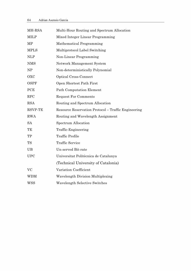
64 Adrian Asensio Garcia
MH-RSA Multi-Hour Routing and Spectrum Allocation
MILP Mixed Integer Linear Programming
MP Mathematical Programming
MPLS Multiprotocol Label Switching
NLP Non-Linear Programming
NMS Network Management System
NP Non-deterministically Polynomial
OXC Optical Cross-Connect
OSPF Open Shortest Path First
PCE Path Computation Element
RFC Request For Comments
RSA Routing and Spectrum Allocation
RSVP-TE Resource Reservation Protocol – Traffic Engineering
RWA Routing and Wavelength Assignment
SA Spectrum Allocation
TE Traffic-Engineering
TP Traffic Profile
TS Traffic Service
UB Un-served Bit-rate
UPC Universitat Politècnica de Catalunya
(Technical University of Catalonia)
VC Variation Coefficient
WDM Wavelength Division Multiplexing
WSS Wavelength Selective Switches
3
References
[Ca12] A. Castro, L. Velasco, M. Ruiz, M. Klinkowski, J. P. Fernández-Palacios, and D. Careglio, "Dynamic Routing and Spectrum (Re)Allocation in Future Flexgrid Optical Networks", Elsevier Computers Networks, 56, 2869-2883, 2012.
[Ch83] V. Chvatal, Linear Programming, Ed. Freeman, 1983.
[Ch92] I. Chamtlac, A. Ganz, and G. Karmi, “Lighpath communications: An approach to high-bandwidth optical WAN’s,” IEEE/ACM Transactions on Networking, vol. 40, no. 7, pp. 1172-1182, Jul. 1992.
[CPLEX] IBM ILOG CPLEX, http://www-01.ibm.com/software/integration /optimization/cplex-optimizer/
[DRAFT1] F. Zhang, O. Gonzalez de Dios, and D. Ceccarelli, "RSVP-TE signaling extensions in support of flexible grid," IETF RFC Draft, Mar. 2012.
[DRAFT2] F. Zhang, X. Zhang, R. Casellas, O. Gonzalez de Dios, and D. Ceccarelli, "GMPLS OSPF-TE extensions in support of flexible-grid in DWDM networks," IETF RFC Draft Mar. 2012.
[FINISAR] Finisar. (2011) Programmable narrow-band filtering using the WaveShaper 1000E and WaveShaper 4000E. white paper. [Online]. Available: http://www.finisar.com
[Fr97] D. Freedman, R. Pisani, and R.Purves, Statistics, 3rd ed. W. W. Norton & Company, 1997.
[G.694] ITU-T. Rec. G.694.1: Spectral grids for WDM applications: DWDM frequency grid, International Telecommunication Union, ITU-T, Jun. 2002.
[Ge11] D.J. Geisler et al., "Bandwidth scalable, coherent transmitter based on parallel synthesis of multiple spectral slices," in Proc. of OFC, los Angeles, USA, Mar. 2011.
[Go10] J. Gonçalves and M. Resende, “Biased random-key genetic algorithms for combinatorial optimization,” J. Heuristics, in press, on-line Aug. 2010.
[Ji10] M. Jinno et al., "Distance-adaptive spectrum resource allocation in spectrum-sliced elastic optical path network," IEEE Commm. Mag.,
66 Adrian Asensio Garcia
vol. 48, no. 8, pp. 138-145, 2010.
[Ki12] D. King, A. Farrel, Y. Li, F. Zhang, and R. Casellas, "Generalized labels for the flexi-grid in lambda-switch-capable (LSC) label switching routers," IETF RFC Draft, Mar. 2012.
[Li11] Y. Li, F. Zhang, and R. Casellas, “Flexible grid label format in wavelength switched optical network,” IETF RFC Draft, Jul. 2011.
[MATLAB] Matlab®, Mathworks® http://www.mathworks.es/products/matlab/
[Ru11] M. Ruiz et al., "Survivable IP/MPLS-Over-WSON multilayer network optimization," J. of Opt. Commun. and Netw., vol. 3, pp. 629-640, 2011.
[RFC2328] J. Moy, "OSPF Version 2," IETF RFC 2328, Apr. 1998.
[RFC3031] E. Rosen, A. Viswanathan, and R. Callon, “Multiprotocol Label Switching Architecture,” IETF RFC 3031, Jan. 2001.
[RFC3209] D. Awduche, L. Berger, D. Gan, T. Li, V. Srinivasan, and G. Swallow, " RSVP-TE: Extensions to RSVP for LSP Tunnels," IETF RFC 3209, Dec. 2001.
[RFC3945] E. Mannie, “Generalized Multi-Protocol Label Switching Architecture,” IETF RFC 3945, Oct. 2004.
[RFC4204] J. Lang, Ed., "Link Management Protocol (LMP)," IETF RFC 4204, Oct. 2005.
[Ve12] L. Velasco et al. “Elastic Spectrum Allocation for Variable Traffic in Flexible-Grid Optical Networks” in Proc. IEEE/OSA Optical Fiber Communication Conference (OFC), 2012.
[Zh11] F. Zhang et al., "Requirements for GMPLS control of flexible grids," IETF RFC Draft, Oct. 2011.